Large language models have changed the world. The OpenAI series of GPT models has led to ChatGPT, which has seen significant adoption in 2023. Next to those closed-source approaches, there has been the emergence of a vast landscape of open source models such as Mistral's 7B and MoE models, the LLaMA family, and others.

But even though there has been a lot of progress training wise, running these models for inference still requires powerful hardware. Even though progress has been impressive (running those LLMs can now often be done on a single GPU-equipped laptop!), we would eventually want such models to be able to run on smartphones and other edge devices.

Late December 2023, a research team from Apple released the LLM in a Flash paper. It "tackles the challenge of efficiently running LLMs that exceed the available DRAM capacity by storing the model parameters on flash memory but bringing them on demand to DRAM" (Alizadeh et al., 2023). In other words, parts of the model are stored in different memory and loaded dynamically, only when they are needed.

In this article, I'm exploring the paper. It begins with why running large language models on edge hardware is difficult. Then, I'm looking at the LLM in a Flash paper and the three main categories for optimization proposed by the authors:

• Reducing the amount of data transferred between flash memory and DRAM by intelligently looking at what parts of the model are needed.
• Improving transfer speed between flash memory and DRAM by intelligently combining data in memory, to transfer larger chunks at once.
• Optimizing data management in DRAM by an intelligent preallocation and memory updating strategy.

Then, I briefly summarize results. This way, you'll learn why optimizing memory management can really be beneficial if you want to run large language models on memory-constrained hardware.

Let's go! 😎

Running large language models on GPUs is costly

First, let's set the stage by exploring why running large language models on edge hardware is costly. For that, we'll need to take a look at how GPU memory works. I found this great article by Thushan Ganegedara from June 2023 which explains the basics very well together with the CUDA Programming Guida (Nvidia, n.d.).

Let's see:

• Ignoring a variety of caches, memory-wise, a GPU has High-Bandwidth Memory (HBM) - which is a type of Dynamic random-access memory (DRAM). It also has Static RAM (SRAM) and local, thread-based registers.
• HBM is largest (and typically what you see when you're executing nvidia-smi), with large GPUs such as A100s often in the range of 40-80 GB (Dao et al., 2022). It is essentially the GPU's global memory.
• This is followed by Static RAM, which is fast but small memory assigned to a streaming multiprocessor (SM; a part of your GPU which processes blocks of threads; Nvidia, n.d.). On an A100 GPU, it has a size of approximately 192KB (Dao et al., 2022) per SM. It serves as shared memory between threads within an SM, or regional memory if you will, following the analogies presented in this list.
• And finally, a GPU also has registers, which are individually allocated to threads for executing their tasks and can hence be considered to be local memory.

Speed vs size

In terms of speed vs size:

• HBM trades-off speed for size; it is relatively slow with 1.5-2.0TB/s (Dao et al., 2022).
• SRAM does the opposite. While very small, it is also very fast with speeds around 19TB/s (Dao et al., 2022). That way, local operations can benefit of insanely fast speeds when requiring inter-thread memory.

Using a model for inference

Okay, now that we understand what these components are, let's sketch how a model is typically used for inference from the perspective of the GPU:

1. First of all, the model weights are loaded into HBM (i.e. into DRAM, which is the more general term used by the LLM in a Flash authors). If you're getting CUDA OOM errors when loading (or training) any model, the size of your model weights or the amount of data passed through your model is larger than HBM and hence some data cannot be allocated.
2. The inference process is started. For a layer, the weights matrix is taken from HBM. However, it is typically larger than what fits in SRAM. Let's point toward the great article by Thushan Ganegedara again: only the cell(s) from the matrix necessary to perform the compute operation in a thread (the kernel function) are loaded into the SM's SRAM. When computation is done, the results are written to HBM and the next step is executed (starting at 2 again).

In order to load specific models, significant amounts of GPU RAM (i.e. HBM, i.e. DRAM) are required. For example, for Mistral 7B, a minimum of 16 GB is what you'll need to make it run in the first place, although 64GB is recommended (Hardware Corner, 2023).

The same is true for CPU-based inference at the edge

The setting above discusses inference when done on GPUs. Let's now assume that you want to run your model at the edge. That is, you're not interested in running the model in a central place (such as in the cloud), where requests to the model are queued and where responses are sent back.

No, you want to run the model on the device yourself, such as your smartphone. This is a requirement for making privacy friendly LLM applications, such as assistants which learn anything about you. You don't want that on some third-party server.

Typically, you can load your models into the GPU but inference is often also done on CPU because no compatible GPUs are available. Here, too, your DRAM comes into play, although it's not HBM - but probably DDR based RAM.

Dynamic random access memory (DRAM) is a type of semiconductor memory that is typically used for the data or program code needed by a computer processor to function. DRAM is a common type of random access memory (RAM) that is used in personal computers (PCs), workstations and servers. Random access allows the PC processor to access any part of the memory directly rather than having to proceed sequentially from a starting place. RAM is located close to a computer's processor and enables faster access to data than storage media such as hard disk drives and solid-state drives (Techtarget, 2019).

It does not matter whether you're running the model on your CPU or on your GPU, the same amounts of memory (in DDR DRAM and if running on GPU also on your GPU's HBM based DRAM) are necessary for running the models successfully. The problem is that these large amounts are typically unavailable on edge devices: as far as I know, some of the latest iPhones have 8GB of RAM, meaning that Mistral 7B cannot run on them as we speak.

LLM in a Flash paper

The LLM in a Flash paper written by Alizadeh et al. (2023) is an attempt to improve this situation. The authors, which are all working for Apple (I am thus not surprised by their interest in this problem), propose a core idea for allowing models larger than available DRAM to run on edge devices:

What if it is possible to store all model weights in flash memory, then load the critical weights into DRAM, followed by dynamically loading the other weights when necessary?

The idea looks as follows:

• There is some flash memory, which is rather slow compared to the other memory components (even slower than regular DRAM) but sufficiently large to store all model weights.
• Critical weights of the LLM (in the case of large language models, these are the weights of the attention parts, for example) are loaded to DRAM all the time, and a priori. This is followed by loading noncritical weights only when necessary, done dynamically.
• The GPU or CPU then uses these weights for computation and then discards weights no longer necessary from memory, going back to step 2, until the inference process is complete.

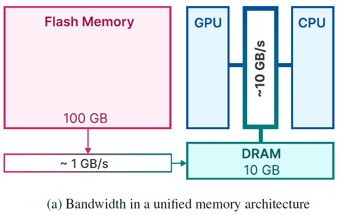
The memory architecture as proposed by Alizadeh et al. (2023).

While quite a good idea (as results show that it is feasible to run models larger than available DRAM this way), the authors describe some roadblocks (Alizadeh et al., 2023). The roadblocks are primarily related to the slow transfer speed between flash memory and the size of DRAM itself. They propose three main strategies (with various sub strategies) to deal with those roadblocks:

1. Reducing the amount of data transferred.
2. Improving transfer throughput with chunk sizes.
3. Optimizing data management in DRAM.

Let's analyze these in more detail.

Reducing the amount of data transferred

Transfer speed wise, the path between flash memory and DRAM is a bottleneck. One very simple solution to experience lower impact of this bottleneck is reducing the amount of data transferred from flash memory into DRAM. In the paper, the authors describe that it is in fact possible to do this without compromising on model quality.

They describe three sub strategies which they tested for doing so:

1. A selective persistence strategy, which means to only load the weights that are necessary at all times up front, while dynamically loading the noncritical ones.
2. Anticipating ReLU sparsity for determining which weights need to be loaded dynamically, allowing you to be more selectively persistent.
3. Keeping active neurons in memory while discarding others based on a sliding window, i.e. sliding window data management.

Selective Persistence Strategy

Firstly, the authors propose to be selective when choosing what weights to persist - i.e., to store in DRAM.

We opt to retain the embeddings and matrices within the attention mechanism of the transformer constantly in RAM. For the Feed-Forward Network (FFN) portions, only the non-sparse segments are dynamically loaded into DRAM as needed (Alizadeh et al., 2023).

According to the authors, for the OPT 7B and Falcon 7B models, this means that approximately 1/3 of the model is stored in DRAM by default. The other 2/3 is loaded dynamically.

This already reduces the memory requirements quite significantly, although we're not there yet, as we haven't loaded all necessary components at this point in order to complete our forward pass.

Anticipating ReLU Sparsity

Okay, good. We need to load the other weights dynamically. But how do we do that? One way is by benefiting from the inherent sparsity of feed-forward layers in LLMs, due to the ReLU activation function.

The ReLU activation function naturally induces over 90% sparsity in the FFN’s intermediate outputs, which reduces the memory footprint for subsequent layers that utilize these sparse outputs (Alizadeh et al., 2023).

The authors propose to "employ a low-rank predictor to identify the zeroed elements post-ReLU". What this means can be seen in the image below (and low-rank benefits are explained in the context of LoRA here).

What is happening is that the model is slightly altered. A low-rank predictor (which are essentially two matrices of dimensionality N x r and r x M where r is way smaller than both N and M) is added to the output of each attention layer (next to the feedforward layer, which is there already). The low-rank nature means that a N x M matrix can be computed by multiplying both matrices without adding many extra parameters to the model (which would offset the benefits). In other words, by adding these layers, extra learning behavior can be added to the model.

But what learning behavior?

More interesting than the fact that the predictor is low-rank is that it ends in a Sigmoid-activated output (i.e. all outputs are between 0 and 1). Combined with a threshold (if sigmoid(prediction) > 0.5, the class outcome is 1; it is 0 otherwise) this leads you a classification: will this neuron be active or silent? Since the Tensor has the same dimensionality as that of the ReLU-activation (both M), this prediction can be used as a mask for what neurons will be active.

And only these weights will be loaded dynamically from flash memory into DRAM before the up projection is computed.

In other words, the selective persistence strategy means that 1/3 of the used 7B models are loaded up front; anticipating ReLU sparsity will determine which other amount of the 2/3rd is loaded when needed.

Low rank predictor besides the FC up projection (Alizadeh et al., 2023).

Sliding Window Data Management

Anticipating ReLU sparsity will instruct you what weights to load dynamically. Naïvely, if your predictor tells you to load specific neurons (and hence weights), you could load all of them from flash memory into DRAM.

But what if certain weights were already loaded?

It would be inefficient, a waste even, to load them another time.

The same is true for keeping weights in DRAM if they are not necessary at a specific point in time.

That's why the authors propose using a sliding window technique for managing what neurons are active and hence what weights are present in DRAM at every time during the inference process.

We define an active neuron as one that yields a positive output in our predictive model. Our approach focuses on managing neuron data by employing a Sliding Window Technique. This methodology entails maintaining neuron data only for a recent subset of input tokens in the memory (Alizadeh et al., 2023).

This sliding window technique can be compared with just-in-time loading and works as follows:

• A sliding window of some tokens (a subset of the whole sequence) is defined. For example, for the sequence 0:l, 0:k is a sliding window over some amount of tokens k << l. Then, s_agg(k) is the amount of neuron data stored in DRAM for the sliding window. The goal is to keep s_agg(k) approximately equal all the time, even when sliding the window across the sequence.
• Avoiding loading tokens another time: for the next 'slide' of the window (i.e., for 1:k+1), it is possible to predict what new neurons must be loaded via neuron activation prediction (using the low-rank predictor). Doing so, it is easy to follow that only s_agg(k+1) - s_agg(k) new neurons need to be loaded from DRAM, as can be seen in the image below (the neurons in dark blue are loaded; the neurons from the initial window are kept in memory). Interestingly, what the authors found was that decreasingly extra neurons need to be loaded for longer sequences, which means that the sliding window approach is really useful to only load neurons just in time.
• Dropping neurons that are no longer necessary: similarly, it is possible to drop neurons when they are no longer necessary at a specific 'sliding configuration' (in the image below, for the current position, the neurons in pink). The authors propose an intelligent mechanism for doing so when managing DRAM, which we'll come back to later.

By loading only necessary neuron data with a sliding window, it is possible to load the neurons precisely when you need them, while total amount of DRAM usage can be kept as low as possible by performing deletes of non-necessary neurons as well.

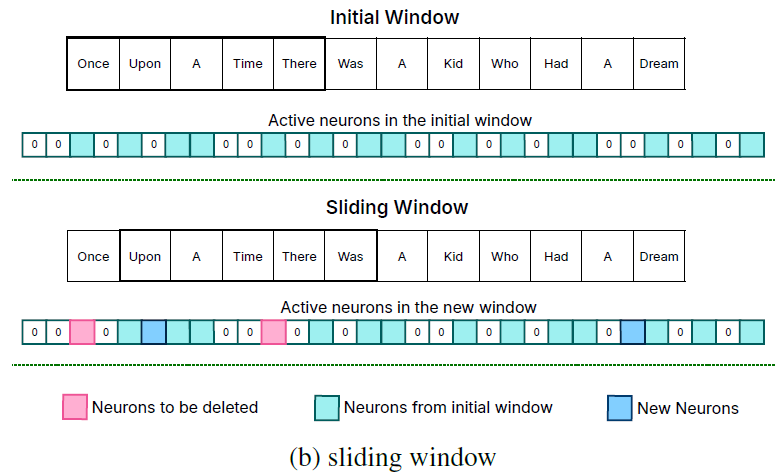
Sliding window data management (Alizadeh et al., 2023).

Improving transfer throughput with chunk sizes

Also known as reading larger chunks. Interestingly, the authors found that a large chunk of data is transferred from flash memory faster compared to a few smaller chunks.

Flash memory systems perform optimally with large sequential reads. For instance, benchmarks on an Apple MacBook Pro M2 with 2TB flash demonstrate speeds exceeding 6GiB/s for a 1GiB linear read of an uncached file. However, this high bandwidth is not replicated for smaller, random reads due to the inherent multi-phase nature of these reads, encompassing the operating system, drivers, interrupt handling, and the flash controller, among others (Alizadeh et al., 2023).

For this reason, the authors have proposed two strategies for making chunk sizes larger - while thus attempting to improve transfer throughput. The first is bundling matrix columns and rows; the other is coactivation bundling.

Bundling matrix columns and rows

The first strategy, bundling matrix columns and rows, essentially boils down to the observation that in Transformer FFN projection layers the activation of neuron i boils down to "the usage of the ith column from the upward projection and the ith row from the downward projection".

Hence, if neuron i is predicted to be active, both weights need to be loaded. Then, why not combine them into a larger chunk, increasing throughput of the neuron? That is what is meant with bundling matrix columns and rows.

Consequently, by storing these corresponding columns and rows together in flash memory, we can consolidate the data into larger chunks for reading (Alizadeh et al., 2023).

Coactivation bundling

The second strategy, which failed, is related to bundling weights of neurons that coactivate - or, in their words,

We had a conjecture that neurons may be highly correlated in their activity patterns, which may enable further bundling (Alizadeh et al., 2023).

To validate this conjecture, the behavior of neurons over a validation set was computed. It was indeed the case that a power law behavior was followed (i.e., where some neurons activate very often, while there is a long tail of not-so-often activating neurons as well). Now, if you call the neurons that coactivate with a particular neuron its closest friends, then you can bundle them together for the often-activating neurons and loading them as a chunk - potentially reducing transfer.

Unfortunately, that did not work as expected, because

[T]his resulted in loading highly active neurons multiple times [due to the fact that a small set of neurons is active most of the times, and hence is loaded again and again because they also have closest friends that are very active] and the bundling worked against our original intention. It means, the neurons that are very active are ‘closest friend‘ of almost everyone (Alizadeh et al., 2023).

For this reason, this strategy was omitted in further experiments.

Optimized Data Management in DRAM

Transferring less data from flash memory to DRAM and improving throughput during transfer are two strategies which focus on moving data from A to B. The third strategy proposed by Alizadeh et al. (2023) is optimizing data management in DRAM itself. In other words, if you've moved data from A to B, gains are possible if management of B is done well. Let's take a look at how this works.

If you are transferring (parts of) the weights of your model from flash memory into DRAM, you're effectively going to reallocate parts of the existing weights in memory in order to structure things well. Also, you often need to allocate more DRAM before you can actually put the data there. This incurs time and hence slows down the inference process. For this reason, Alizadeh et al. (2023) propose to:

1. Preallocate all necessary memory up front.
2. Establishing a management structure for DRAM.

This management structure uses a few variables to:

1. Check which neurons are no longer necessary before deleting them.
2. Replacing the 'gaps' within the memory structure with the existing elements, so that they again nicely stack together.
3. Appending new neurons to the end of the stack.

Results

While I would refer to the LLM in a Flash paper for a more thorough discussion of the results, it's interesting to note that:

The practical outcomes of our research are noteworthy. We have demonstrated the ability to run LLMs up to twice the size of available DRAM, achieving an acceleration in inference speed by 4-5x compared to traditional loading methods in CPU, and 20-25x in GPU (Alizadeh et al., 2023).

In other words:

• By intelligently loading and using model weights, significant memory savings can be achieved, meaning that models that are approximately 2x as large as available DRAM can still run on the particular device
• CPU-wise, 4-5x speedups are achieved. Even more impressive, 20-25x GPU speedups are achieved.

References

Alizadeh, K., Mirzadeh, I., Belenko, D., Khatamifard, K., Cho, M., Del Mundo, C. C., ... & Farajtabar, M. (2023). LLM in a flash: Efficient Large Language Model Inference with Limited Memory. arXiv preprint arXiv:2312.11514.

Ganegedara, T. (2023, June 15). Hey GPU, what’s up with my matrix? Medium. https://towardsdatascience.com/hey-gpu-whats-up-with-my-matrix-cb7f6d7ae7d6

Dao, T., Fu, D., Ermon, S., Rudra, A., & Ré, C. (2022). Flashattention: Fast and memory-efficient exact attention with io-awareness. Advances in Neural Information Processing Systems, 35, 16344-16359.

Hardware Corner. (2023, December 12). Mistral LLM: All versions & hardware requirements – Hardware corner. Refurbished Computers: Laptops, Desktops, and Buying Guides. https://www.hardware-corner.net/llm-database/Mistral/

Techtarget. (2019, November 7). What is DRAM (Dynamic random access memory)? How does it work? Storage. https://www.techtarget.com/searchstorage/definition/DRAM

Nvidia. (n.d.). CUDA C++ programming guide. NVIDIA Documentation Hub - NVIDIA Docs. https://docs.nvidia.com/cuda/cuda-c-programming-guide/index.html