CLIP: how it works, how it's trained and how to use it
December 22, 2023 by Chris
When you started with acquiring knowledge about deep learning methods, neural network classifiers were probably part of your learnings. These networks, which are trained on datasets which have many samples for a limited amount of classed, are strongly supervised.
But they don't scale well to samples that go beyond the distribution present within your training set.
And neither do they allow you to reuse them on different classification problems. When trained properly, they work well for the problem they were trained for - but that's it.
In 2021, researchers at OpenAI looked into methods to solve this. Specifically, they wondered if it would be possible to build a mechanism for zero-shot classification, in other words, a method that works on a variety of examples without explicit training nor the provisioning of similar examples in the prompt at inference time.
And yes, this turned out to be possible! In this article, we're taking a look at CLIP, which enables zero-shot behavior by being trained on text and images... at the same time.
Problems with directly mapping images to text
Building a zero-shot classifier can be done in multiple ways; one architecture is not necessarily better than another. When designing such architectures, it is common to use the Transformer (Vaswani et al., 2017). It is the state of the art in NLP these days. In fact, many modern language models can originally be traced back to (parts) of this architecture.
In one of their first attempts, the OpenAI researchers tried jointly training an image and text model in prediction image captions:
Our initial approach, similar to VirTex, jointly trained an image CNN and text transformer from scratch to predict the caption of an image. However, we encountered difficulties efficiently scaling this method (Radford et al., 2021).
Unfortunately, that didn't work well. According to the authors, the problem which the model attempted solving - effectively a predictive problem - is a really difficult one:
[The model tries] to predict the exact words of the text accompanying each image. This is a difficult task due to the wide variety of descriptions, comments, and related text that co-occur with images (Radford et al., 2021).
CLIP: Contrastive Language-Image Pretraining
Instead, they argue, a contrastive approach may work better. Imagine that you are teaching a child what a banana looks like. Often, you show it a banana, saying "banana!". Then, you alternate with other fruits ("other fruit!"), from which the child eventually learns to distinguish bananas from these fruits.
In other words, you're employing a contrastive learning strategy.
Contrastive learning is an approach to learning that focuses on extracting meaningful representations by contrasting positive and negative pairs of instances (Encord, 2023).
Now that we understand what contrastive learning is, let's take a look at CLIP itself.
CLIP design
CLIP, or Contrastive Language-Image Pretraining , is a model trained jointly on pairs of languages and images. There's a text encoder which encodes texts and an image encoder which encodes into shared embedding space with dimensionality d_e. Before looking at how CLIP is trained, let's take a look at these individual components.
Encoding text
Text wise, byte-pair encodings with a maximum sequence length of 76 are fed through a Transformer, which is from the Radford et al. (2019) paper - so GPT-2. Activations of the highest layer are considered as the textual feature representations. These are then linearly projected into embedding space with dimensionality d_e.
The text encoder is a Transformer (Vaswani et al., 2017) with the architecture modifications described in Radford et al. (2019) (Radford et al., 2019)
Encoding images
Something similar is done with the image batches. They are also encoded and projected into embedding space with dimensionality d_e. However, in their work, the authors were a bit more experimental with regards to images compared to text. Instead of using just one Transformer (GPT-2), they used two different architectures to see which one worked best. Specifically, they used a series of modified ResNets and a series of Vision Transformers (as introduced by Dosovitskiy et al. in 2020. The latter ones worked better, with one trained at higher image resolution in particular. Radford et al. mention that if they're talking about CLIP, they mean the combination of GPT-2 with that specific Vision Transformer.
Training CLIP
The magic of CLIP happens when the two modalities are combined in the forward pass of which the outcome is used for optimization. I must admit, it was slightly complex to understand at first, but the beauty of it became really clear later.
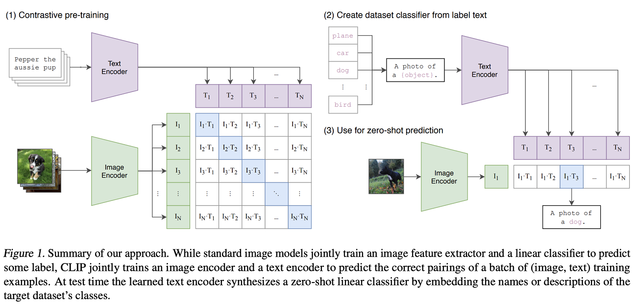
Let's take a look at the image above. Currently, you know that the two batches - when fed through both transformers - both have the same shape at this point in time: there are N images/texts of dimensionality d_e, so [N, d_e] is the shape of both the images and the texts.
Visually, they are the purple row and green column in the left part of the above image.
Forward pass and computing similarity
Subsequently, the the following happens:
-
- For each pair of images and texts (represented by two vectors per pair, one for the image; another for the text), vector similarity is computed. This is done by first L2 normalizing the vectors, after which cosine similarity is computed (by means of dot products, which leads to equal results). This leads to a similarity matrix.
-
- Based on similarities, a symmetric loss is computed. What this means is that a loss function is computed over the vertical and horizontal axis, where the logits of the matrix are compared with some labels (Radford et al., 2021).
Given a batch of N (image, text) pairs, CLIP is trained to predict which of the N × N possible (image, text) pairings across a batch actually occurred. To do this, CLIP learns a multi-modal embedding space by jointly training an image encoder and text encoder to maximize the cosine similarity of the image and text embeddings of the N real pairs in the batch while minimizing the cosine similarity of the embeddings of the N2 − N incorrect pairings. We optimize a symmetric cross entropy loss over these similarity scores (Radford et al., 2021).
CLIP symmetric loss - how does it work?
This is the pseudocode of CLIP's symmetric loss function (Radford et al., 2021):
# symmetric loss function
labels = np.arange(n)
loss_i = cross_entropy_loss(logits, labels, axis=0)
loss_t = cross_entropy_loss(logits, labels, axis=1)
loss = (loss_i + loss_t)/2
In other words, symmetric here means that it's just the average over cross-entropy loss computed between some labels and the logits across two axes.
But what confused me was how said loss can be computed over the logits while labels are defined as np.arange(n).
I've finally found out. Let me explain.
It begins with understanding what is actually meant with computing np.arange:
Return evenly spaced values within a given interval (NumPy, n.d.).
In other words, this gives us a list of integers, with n=3 e.g. [0, 1, 2]. Then, I got even more confused. How can each integer ever be used to compare with some logits vector (each row or column of the similarity matrix)?
After quite a bit of searching, I looked again at the image provided above. As you can see, the correct pairs of texts and images represent a diagonal. Index-wise, this means that each pair can be found at [i, i], where i is in the range between 0 and n. In other words, np.arange(n) represents the true indices of the diagonal: np.arange(3) = np.array([0, 1, 2]). This is equal to the positions [(0, 0), (1, 1), (2, 2)]. The diagonal!
When I understood that, I was a step closer. But what I still did not understand is how one integer value (for example, 0) could be used in computing the loss when compared with a vector.
Then I learned that cross-entropy loss in many deep learning frameworks (such as PyTorch) accepts an integer as a target, being a class index:
The target that this criterion expects should contain either (...) class indices in the range [0, C) where C is the number of classes (PyTorch, n.d.).
Internally, PyTorch converts the class index to a one-hot encoded representation. In other words, class index 3 for 5 possible classes means that the corresponding label becomes [0, 0, 0, 1, 0] after conversion. After that, it is possible to compute cross-entropy loss between the logits and the label - because the two tensors can be compared.
CLIP loss - an example
Let's now make this even more clear with an example - it is the core of CLIP, after all, so it's important to understand thoroughly.
Suppose that we're having this similarity matrix, which are the logits - the dot products produced as a similarity measure for every (text, vector) combination:
| t1 | t2 | t3 | |
|---|---|---|---|
| i1 | 0.9 | 0.2 | 0.1 |
| i2 | 0.3 | 0.8 | 0.2 |
| i3 | 0.1 | 0.4 | 0.7 |
You can clearly see that the diagonal has the highest values. This makes sense, because the diagonal contains the true pairs (t1, i1), (t2, i2) and (t3, i3). And that is why the original paper defines labels as np.arange(n): this numeric range contains the correct pairs 0, 1 and 2.
Subsequently, CLIP loss is computed across both dimensions: once for the text/images pairs and another time for the image/texts pairs.
In both directions, you'd expect to find this:
- For the first pair:
[1 0 0]. - For the second pair:
[0 1 0]. - For the third pair:
[0 0 1].
Suppose you're computing the first loss, over axis=0, so downwards across all rows. You're passing index = 0 for the first row, index = 1 for the second, and so on; in other words, passing [1 0 0], [0 1 0] et cetera. In other words, when computing loss, you'll compare [0.9 0.2 0.1] with [1 0 0], [0.3 0.8 0.2] with [0 1 0] and so on. This leads to a loss: there are small but significant differences between the logits and the expected values. There is no perfect diagonal (i.e., an identity matrix) after all, especially at first, when the network is initialized pseudo-randomly (or with different initialization schemes resembling it). But we're trying to get there, so we compute the loss over axis=0!
Then, you'll do the same over axis=1 so horizontally across all columns. You finally combine both losses and divide them by 2, so that the losses over the horizontal and vertical axes contribute equally to how wrong the model is.
This is then used in the backwards pass leading to model optimization.
Eventually, when trained, the best similarity matrix for the passed batch is an identity matrix. However, that would probably happen only in theory. In practice, it'll never be that perfect, but results have shown that they are good enough for practical use!
Using CLIP
Let's now take a look at a few use cases for CLIP:
- Performing zero-shot classification. In other words, building a classifier with text pairs - without requiring any upfront examples during inference.
- Building an image search engine, where you'll be able to find images matching a specific text in your dataset or vice-versa; texts matching a specific image.
- Finetuning the model to your own dataset, if necessary.
Zero-shot classification
Let's revisit the image. Above, we discussed what's visualized under (1) - contrastive pre-training. When OpenAI was done training, they found a model that is capable to understand relevance between a text and an image. This allows you to perform zero-shot classification, which is defined as follows:
Zero-shot (...) classification is a task in natural language processing where a model is trained on a set of labeled examples but is then able to classify new examples from previously unseen classes. (HuggingFace, n.d.)
Even better, because of the fact that it was trained on pairs of texts and images, it's possible to create any classifier you want! Let's take a look.
What we're seeing here under (2) and (3) is the following:
- A text set of everyday objects is generated:
plane, car, dog, ..., bird. This set is subsequently used to format newer strings, such asA photo of a car. These are passed to the trained text encoder, meaning that they are converted into vectors that have the dimensionality of the embedding space. - The same is done with an image. For example, in the image above, you'll see that it's a photo of a dog. Here, too, the image is passed through the trained encoder model (the ViT) and converted into an embedding vector having the same dimensionality of the embedding space.
- Then, similarity scores are computed by taking the dot product between each text embedding and the image embedding (recall that this equals cosine similarity in this case). This leads to logits; like during training, the highest logit is the most probable class. Of course, it is possible to compute a Softmax activation over these logits to ensure that the sum of them equals 1, but this is not necessary.
Indeed, in our case, the third textual input is most likely: it's a photo of a dog.
What this means is that you'll be able to compose a textual set of any object you'd like (for example, banana, apple and orange), pass it through the trained text encoder, pass an image through the trained image encoder, compute similarity and find the most probable class. A true zero-shot image classifier!
If you want to create such a classifier yourself, make sure to read this article.
Image search engine
There's another interesting CLIP use case: it can be used as an image search engine. Suppose that you have a dataset of images, say, 1000 photos that you'd like to search through. Using CLIP, it would not be too difficult to build a web page that takes a textual input (for example, "a yellow car in New York City") and have it return images which are similar.
Finetuning to your own datasets
CLIP was trained on a large-scale dataset, but the objects in the images were relatively common and taken from specific angles (as you would expect with regular images). It is hence difficult to use the model for use cases which require other angles, such as satellite images.
Similar to any large model, it's possible to fine-tune CLIP with your own dataset. Here is an example which demonstrates how to do that using satellite imagery.
Today, you've learned to understand CLIP better: what its components are, how it is trained, and how it can be used. I hope the article has helped you gain a deeper understanding about this model. Thanks for reading - and let's connect if you have any questions or remarks!
References
Radford, A., Kim, J. W., Hallacy, C., Ramesh, A., Goh, G., Agarwal, S., ... & Sutskever, I. (2021, July). Learning transferable visual models from natural language supervision. In International conference on machine learning (pp. 8748-8763). PMLR.
Encord. (2023, July 14). Full guide to contrastive learning. Data Engine for AI Model Development | Encord. https://encord.com/blog/guide-to-contrastive-learning
NumPy. (n.d.). Numpy.arange — NumPy v1.26 manual. https://numpy.org/doc/stable/reference/generated/numpy.arange.html
PyTorch. (n.d.). CrossEntropyLoss — PyTorch 2.1 documentation. https://pytorch.org/docs/stable/generated/torch.nn.CrossEntropyLoss.html
HuggingFace. (n.d.). Zero-shot classification. Hugging Face – The AI community building the future. https://huggingface.co/tasks/zero-shot-classification
Vaswani, A., Shazeer, N., Parmar, N., Uszkoreit, J., Jones, L., Gomez, A. N., ... & Polosukhin, I. (2017). Attention is all you need. Advances in neural information processing systems, 30.
Radford, A., Wu, J., Child, R., Luan, D., Amodei, D., & Sutskever, I. (2019). Language models are unsupervised multitask learners. OpenAI blog, 1(8), 9.
Dosovitskiy, A., Beyer, L., Kolesnikov, A., Weissenborn, D., Zhai, X., Unterthiner, T., ... & Houlsby, N. (2020). An image is worth 16x16 words: Transformers for image recognition at scale. arXiv preprint arXiv:2010.11929.

Hi, I'm Chris!
I know a thing or two about AI and machine learning. Welcome to MachineCurve.com, where machine learning is explained in gentle terms.
Getting started
Foundation models
Learn how large language models and other foundation models are working and how you can train open source ones yourself.
Keras
Keras is a high-level API for TensorFlow. It is one of the most popular deep learning frameworks.
Machine learning theory
Read about the fundamentals of machine learning, deep learning and artificial intelligence.
Most recent articles
January 2, 2024
What is Retrieval-Augmented Generation?
December 27, 2023
In-Context Learning: what it is and how it works
December 22, 2023
CLIP: how it works, how it's trained and how to use it
Article tags
Most popular articles
February 18, 2020
How to use K-fold Cross Validation with TensorFlow 2 and Keras?
December 28, 2020
Introduction to Transformers in Machine Learning
December 27, 2021
StyleGAN, a step-by-step introduction
July 17, 2019
This Person Does Not Exist - how does it work?
October 26, 2020
Your First Machine Learning Project with TensorFlow 2.0 and Keras
Connect on social media
Connect with me on LinkedIn
To get in touch with me, please connect with me on LinkedIn. Make sure to write me a message saying hi!
Side info
The content on this website is written for educational purposes. In writing the articles, I have attempted to be as correct and precise as possible. Should you find any errors, please let me know by creating an issue or pull request in this GitHub repository.
All text on this website written by me is copyrighted and may not be used without prior permission. Creating citations using content from this website is allowed if a reference is added, including an URL reference to the referenced article.
If you have any questions or remarks, feel free to get in touch.
TensorFlow, the TensorFlow logo and any related marks are trademarks of Google Inc.
PyTorch, the PyTorch logo and any related marks are trademarks of The Linux Foundation.
Montserrat and Source Sans are fonts licensed under the SIL Open Font License version 1.1.
Mathjax is licensed under the Apache License, Version 2.0.