ReLU, Sigmoid and Tanh: today's most used activation functions

Today's deep neural networks can handle highly complex data sets. For example, object detectors have grown capable of predicting the positions of various objects in real-time; timeseries models can handle many variables at once and many other applications can be imagined.

The question is: why can those networks handle such complexity. More specifically, why can they do what previous machine learning models were much less capable of?

There are many answers to this question. Primarily, the answer lies in the depth of the neural network - it allows networks to handle more complex data. However, a part of the answer lies in the application of various activation functions as well - and particularly the non-linear ones most used today: ReLU, Sigmoid and Tanh.

In this blog, we will find out a couple of things:

• What an activation function is;
• Why you need an activation function;
• An introduction to the Sigmoid activation function;
• An introduction to the Tanh, or tangens hyperbolicus, activation function;
• An introduction to the Rectified Linear Unit, or ReLU, activation function.

Are you ready? Let's go! :-)

Update 17/Jan/2021: checked the article to ensure that it is up to date in 2021. Also added a short section with the key information from this article.

In short: the ReLU, Sigmoid and Tanh activation functions

In today's deep learning practice, three so-called activation functions are used widely: the Rectified Linear Unit (ReLU), Sigmoid and Tanh activation functions.

Activation functions in general are used to convert linear outputs of a neuron into nonlinear outputs, ensuring that a neural network can learn nonlinear behavior.

Rectified Linear Unit (ReLU) does so by outputting x for all x >= 0 and 0 for all x < 0. In other words, it equals max(x, 0). This simplicity makes it more difficult than the Sigmoid activation function and the Tangens hyperbolicus (Tanh) activation function, which use more difficult formulas and are computationally more expensive. In addition, ReLU is not sensitive to vanishing gradients, whereas the other two are, slowing down learning in your network. Also known to generalize well, it is unsurprising to see that ReLU is the most widely used activation function today.

What is an activation function?

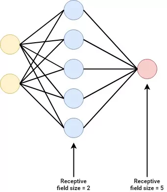
You do probably recall the structure of a basic neural network, in deep learning terms composed of densely-connected layers:

In this network, every neuron is composed of a weights vector and a bias value. When a new vector is input, it computes the dot product between the weights and the input vector, adds the bias value and outputs the scalar value.

...until it doesn't.

Because put very simply: both the dot product and the scalar additions are linear operations.

Hence, when you have this value as neuron output and do this for every neuron, you have a system that behaves linearly.

And as you probably know, most data is highly nonlinear. Since linear neural networks would not be capable of e.g. generating a decision boundary in those cases, there would be no point in applying them when generating predictive models.

The system as a whole must therefore be nonlinear.

Enter the activation function.

This function, which is placed directly behind every neuron, takes as input the linear neuron output and generates a nonlinear output based on it, often deterministically (i.e., when you input the same value twice, you'll get the same result).

This way, with every neuron generating in effect a linear-but-nonlinear output, the system behaves nonlinearly as well and by consequence becomes capable of handling nonlinear data.

Activation outputs increase with input

Neural networks are inspired by the human brain. Although very simplistic, they can be considered to resemble the way human neurons work: they are part of large neural networks as well, with synapses - or pathways - in between. Given neural inputs, human neurons activate and pass signals to other neurons.

The system as a whole results in human brainpower as we know it.

If you wish to resemble this behavior in neural network activation functions, you'll need to resemble human neuron activation as well. Relatively trivial is the notion that in human neural networks outputs tend to increase when stimulation, or input to the neuron, increases. By consequence, this is also often the case in artificial ones.

Hence, we're looking for mathematical formulae that take linear input, generate a nonlinear output and increase or remain stable over time (a.k.a.,

Towards today's prominent activation functions

Today, three activation functions are most widely used: the Sigmoid function, the Tangens hyperbolicus or tanh and the Rectified Linear Unit, or ReLU. Next, we'll take a look at them in more detail.

Sigmoid

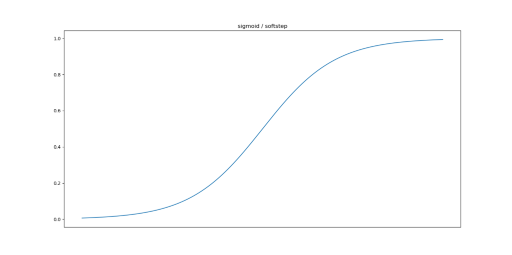
Below, you'll see the (generic) sigmoid function, also known as the logistic curve:

Mathematically, it can be represented as follows:

[mathjax]

\begin{equation} y: f(x) = \frac{1}{1 + e^{-x}} \end{equation}

As you can see in the plot, the function slowly increases over time, but the greatest increase can be found around \(x = 0\). The range of the function is \((0, 1)\); i.e. towards high values for \(x\) the function therefore approaches 1, but never equals it.

The Sigmoid function allows you to do multiple things. First, as we recall from our post on why true Rosenblatt perceptrons cannot be created in Keras, step functions used in those ancient neurons are not differentiable and hence gradient descent for optimization cannot be applied. Second, when we implemented the Rosenblatt perceptron ourselves with the Perceptron Learning Rule, we noticed that in a binary classification problem, the decision boundary is optimized per neuron and will find one of the possible boundaries if they exist. This gets easier with the Sigmoid function, since it is more smooth (Majidi, n.d.).

Additionally, and perhaps primarily, we use the Sigmoid function because it outputs between \((0, 1)\). When estimating a probability, this is perfect, because probabilities have a very similar range of \([0, 1]\) (Sharma, 2019). Especially in binary classification problems, when we effectively estimate the probability that the output is of some class, Sigmoid functions allow us to give a very weighted estimate. The output \(0.623\) between classes A and B would indicate "slightly more of B". With a step function, the output would have likely been \(1\), and the nuance disappears.

Tangens hyperbolicus: Tanh

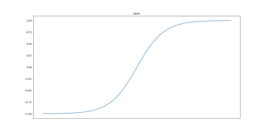
Another widely used activation function is the tangens hyperbolicus, or hyperbolic tangent / tanh function:

It works similar to the Sigmoid function, but has some differences.

First, the change in output accelerates close to \(x = 0\), which is similar with the Sigmoid function.

It does also share its asymptotic properties with Sigmoid: although for very large values of \(x\) the function approaches 1, it never actually equals it.

On the lower side of the domain, however, we see a difference in the range: rather than approaching \(0\) as minimum value, it approaches \(-1\).

Differences between tanh and Sigmoid

You may now probably wonder what the differences are between tanh and Sigmoid. I did too.

Obviously, the range of the activation function differs: \((0, 1)\) vs \((-1, 1)\), as we have seen before.

Although this difference seems to be very small, it might have a large effect on model performance; specifically, how fast your model converges towards the most optimal solution (LeCun et al., 1998).

This is related to the fact that they are symmetric around the origin. Hence, they produce outputs that are close to zero. Outputs close to zero are best: during optimization, they produce the least weight swings, and hence let your model converge faster. This will really be helpful when your models are very large indeed.

As we can see, the tanh function is symmetric around the origin, where the Sigmoid function is not. Should we therefore always choose tanh?

Nope - it comes with a set of problems, or perhaps more positively, challenges.

Challenges of Sigmoid and Tanh

The paper by LeCun et al. was written in 1998 and the world of deep learning has come a long way... identifying challenges that had to be solved in order to bring forward the deep learning field.

First of all, we'll have to talk about model sparsity (DaemonMaker, n.d.). The less complex the model is during optimization, the faster it will converge, and the more likely it is that you'll find a mathematical optimum in time.

And complexity can be viewed as the number of unimportant neurons that are still in your model. The fewer of them, the better - or sparser - your model is.

Sigmoid and Tanh essentially produce non-sparse models because their neurons pretty much always produce an output value: when the ranges are \((0, 1)\) and \((-1, 1)\), respectively, the output either cannot be zero or is zero with very low probability.

Hence, if certain neurons are less important in terms of their weights, they cannot be 'removed', and the model is not sparse.

Another possible issue with the output ranges of those activation functions is the so-called vanishing gradients problem (DaemonMaker, n.d.). During optimization, data is fed through the model, after which the outcomes are compared with the actual target values. This produces what is known as the loss. Since the loss can be considered to be an (optimizable) mathematical function, we can compute the gradient towards the zero derivative, i.e. the mathematical optimum.

Neural networks however comprise many layers of neurons. We would essentially have to repeat this process over and over again for every layer with respect to the downstream ones, and subsequently chain them. That's what backpropagation is. Subsequently, we can optimize our models with gradient descent or a similar optimizer.

When neuron outputs are very small (i.e. \( -1 < output < 1\)), the chains produced during optimization will get smaller and smaller towards the upstream layers. This will cause them to learn very slowly, and make it questionable whether they will converge to their optimum at all: enter the vanishing gradients problem.

A more detailed review on this problem can be found here.

Rectified Linear Unit: ReLU

In order to improve on these observations, another activation was introduced. This activation function, named Rectified Linear Unit or ReLU, is the de facto first choice for most deep learning projects today. It is much less sensitive to the problems mentioned above and hence improves the training process.

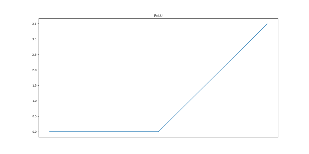
It looks as follows:

And can be represented as follows:

\begin{equation} f(x) = \begin{cases} 0, & \text{if}\ x < 0 \\ x, & \text{otherwise} \\ \end{cases} \end{equation}

Or, in plain English, it produces a zero output for all inputs smaller than zero; and \(x\) for all other inputs. Hence, for all \(inputs <= 0\), it produces zero outputs.

Sparsity

This benefits sparsity substantially: in almost half the cases, now, the neuron doesn't fire anymore. This way, neurons can be made silent if they are not too important anymore in terms of their contribution to the model's predictive power.

Fewer vanishing gradients

It also reduces the impact of vanishing gradients, because the gradient is always a constant: the derivative of \(f(x) = 0\) is 0 while the derivative of \(f(x) = x\) is 1. Models hence learn faster and more evenly.

Computational requirements

Additionally, ReLU does need much fewer computational resources than the Sigmoid and Tanh functions (Jaideep, n.d.). The function that essentially needs to be executed to arrive at ReLU is a max function: \(max(0, x)\) produces 0 when \(x < 0\) and x when \(x >= 0\). That's ReLU!

Now compare this with the formulas of the Sigmoid and tanh functions presented above: those contain exponents. Computing the output of a max function is much simpler and less computationally expensive than computing the output of exponents. For one calculation, this does not matter much, but note that in deep learning many such calculations are made. Hence, ReLU reduces your need for computational requirements.

ReLU comes with additional challenges

This does however not mean that ReLU itself does not have certain challenges:

• Firstly, it tends to produce very large values given its non-boundedness on the upside of the domain (Jaideep, n.d.). Theoretically, infinite inputs produce infinite outputs.
• Secondly, you will face the dying ReLU problem (Jaideep, n.d.). If a neuron's weights are moved towards the zero output, it may be the case that they eventually will no longer be capable of recovering from this. They will then continually output zeros. This is especially the case when your network is poorly initialized, or when your data is poorly normalized, because the first rounds of optimization will produce large weight swings. When too many neurons output zero, you end up with a dead neural network - the dying ReLU problem.
• Thirdly: Small values, even the non-positive ones, may be of value; they can help capture patterns underlying the dataset. With ReLU, this cannot be done, since all outputs smaller than zero are zero.
• Fourthly, the transition point from \(f(x) = 0\) to \(f(x) = x\) is not smooth. This will impact the loss landscape during optimization, which will not be smooth either. This may (slightly albeit significantly) hamper model optimization and slightly slow down convergence.

To name just a few.

Fortunately, new activation functions have been designed to overcome these problems in especially very large and/or very deep networks. A prime example of such functions is Swish; another is Leaky ReLU. The references navigate you to blogs that cover these new functions.

Recap

In this blog, we dived into today's standard activation functions as well as their benefits and possible drawbacks. You should now be capable of making a decision as to which function to use. Primarily, though, it's often best to start with ReLU; then try tanh and Sigmoid; then move towards new activation functions. This way, you can experimentally find out which works best. However, take notice of the resources you need, as you may not necessarily be able to try all choices.

Happy engineering! :-)

References

Panchal, S. (n.d.). What are the benefits of using a sigmoid function? Retrieved from https://stackoverflow.com/a/56334780

Majidi, A. (n.d.). What are the benefits of using a sigmoid function? Retrieved from https://stackoverflow.com/a/56337905

Sharma, S. (2019, February 14). Activation Functions in Neural Networks. Retrieved from https://towardsdatascience.com/activation-functions-neural-networks-1cbd9f8d91d6

LeCun, Y., Bottou, L., Orr, G. B., & Müller, K. -. (1998). Efficient BackProp. Lecture Notes in Computer Science, 9-50. doi:10.1007/3-540-49430-8_2

DaemonMaker. (n.d.). What are the advantages of ReLU over sigmoid function in deep neural networks? Retrieved from https://stats.stackexchange.com/a/126362

Jaideep. (n.d.). What are the advantages of ReLU over sigmoid function in deep neural networks? Retrieved from https://stats.stackexchange.com/questions/126238/what-are-the-advantages-of-relu-over-sigmoid-function-in-deep-neural-networks