Binary Crossentropy Loss with PyTorch, Ignite and Lightning

Training a deep learning model is a cyclical process. First, you feed forward data, generating predictions for each sample. Then, the predictions are compared and the comparison is aggregated into a loss value. Finally, using this loss value, errors are computed backwards using backpropagation and the model is optimized with gradient descent or an adaptive optimizer.

This way, you can train a model that really performs well - one that can be used in practice.

In this tutorial, we will take a close look at using Binary Crossentropy Loss with PyTorch. This loss, which is also called BCE loss, is the de facto standard loss for binary classification tasks in neural networks. After reading this tutorial, you will...

• Understand what Binary Crossentropy Loss is.
• How BCE Loss can be used in neural networks for binary classification.
• Have implemented Binary Crossentropy Loss in a PyTorch, PyTorch Lightning and PyTorch Ignite model.

Let's get to work! 🚀

Using BCELoss with PyTorch: summary and code example

Training a neural network with PyTorch, PyTorch Lightning or PyTorch Ignite requires that you use a loss function. This is not specific to PyTorch, as they are also common in TensorFlow - and in fact, a core part of how a neural network is trained.

Choosing a loss function is entirely dependent on your dataset, the problem you are trying to solve and the specific variant of that problem. For binary classification problems, the loss function that is most suitable is called binary crossentropy loss. It compares the prediction, which is a number between 0 and 1, with the true target, that is either 0 or 1. Having the property that loss increases exponentially while the offset increases linearly, we get a way to punish extremely wrong predictions more aggressively than ones that are close to the target. This stabilizes the training process.

In PyTorch, binary crossentropy loss is provided by means of nn.BCELoss. Below, you'll see how Binary Crossentropy Loss can be implemented with either classic PyTorch, PyTorch Lightning and PyTorch Ignite. Make sure to read the rest of the tutorial too if you want to understand the loss or the implementations in more detail!

Classic PyTorch

Using BCELoss in classic PyTorch is a two-step process:

1. Define it as a criterion.
2. Use it in the custom training loop.

Step 1 - the criterion definition:

criterion = nn.BCELoss()

Step 2 - using it in the custom training loop:

for epoch in range(5):
    for i, data in enumerate(trainloader, 0):
        inputs, labels = data
        optimizer.zero_grad()
    # Forward pass
        outputs = net(inputs)
    # Compute loss
        loss = criterion(outputs, labels)
    # Backward pass
        loss.backward()
    # Optimization
        optimizer.step()

PyTorch Lightning

In Lightning, we can add BCELoss to our training_step, validation_step and testing_step like this to start using Binary Crossentropy Loss:

from torch import nn
import pytorch_lightning as pl

class NeuralNetwork(pl.LightningModule):
  def training_step(self, batch, batch_idx):
    x, y = batch
    x = x.view(x.size(0), -1)
    y_hat = self.layers(x)
    loss = self.bce(y_hat, y)
    self.log('train_loss', loss)
    return loss

PyTorch Ignite

In Ignite, we can add BCELoss as a criterion to the Trainer creation for using Binary Crossentropy Loss. It can be added like this:

from torch import nn

criterion = nn.BCELoss()
trainer = create_supervised_trainer(model, optimizer, criterion, device=device)

Binary Crossentropy Loss for Binary Classification

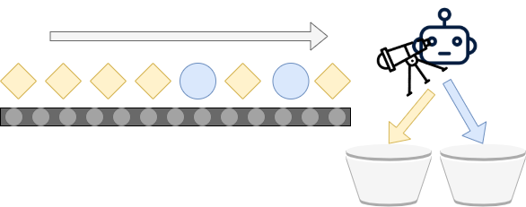
From our article about the various classification problems that Machine Learning engineers can encounter when tackling a supervised learning problem, we know that binary classification involves grouping any input samples in one of two classes - a first and a second, often denoted as class 0 and class 1.

High-level training process

We also know from our article about loss functions and the high-level supervised machine learning process that when you train a neural network, these are the steps that the process will go through:

1. Feeding forward data through the model. The result is a set of predictions with one prediction per input sample.
2. Comparing the predictions with the ground truth. Here, we compute the differences between the prediction and the true sample. We converge these differences in one value, which we call the loss value.
3. Improving the model. By computing the errors backwards by means of backpropagation, we get gradients that we can use to improve the model through optimization.
4. Starting at (1) again. This process is cyclical until a performance threshold has been passed, until time is up or until the process is halted manually.

Sounds like a straight-forward process. But we didn't answer the how with respect to generating differences between predictions and the true sample, and the subsequent convergence of these into a loss value.

Binary crossentropy loss

In fact, there are many loss functions that we can use for this purpose - and each combination of task, variant and data distribution has the best possible candidate.

For binary classification problems, the loss function of choice is the binary crossentropy loss, or the BCELoss, if you will. Don't be scared away by the maths, but it can be defined as follows:

Don't let the maths scare you away... just read on! 😉

Here, t is the target value (either 0.0 or 1.0 - recall that the classes are represented as class 0 and class 1). The prediction p can be any value between zero and one, as is common with the Sigmoid activation function. This function is commonly used to generate the output in the last layer of your neural network when performing binary classification. The log here is the logarithm which generates the exponential properties that make the function so useful.

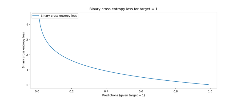
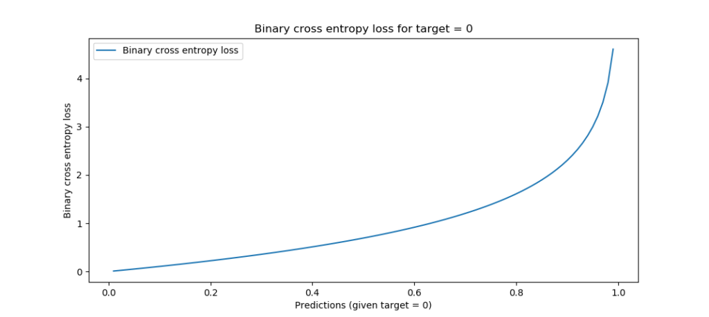
Visualized for the two possible targets and any value for p between 0 and 1, this is what BCE loss looks like:

• 

  Binary crossentropy, target = 1

• 

  Binary crossentropy, target = 0

Indeed:

• If the distance between the target and the prediction is high (e.g. t = 0.0; p = 1.0 or t = 1.0; p = 0.0), loss is highest - infinite, even, for an 1.0 delta.
• There is continuity between all loss values, meaning that all possible values (i.e. [0, 1]) are supported.
• Loss increases exponentially when the difference between prediction and target increases linearly. In other words, predictions that are really wrong are punished more significantly than predictions that are a bit off. This means no craziness when the model is close to optimum values, but quite a shift in weights when it's not.

These properties make binary crossentropy a very suitable loss function for binary classification problems. Let's now take a look at how we can implement it with PyTorch and its varieties.

Implementing Binary Crossentropy Loss with PyTorch

In this section, we'll see a step-by-step approach to constructing Binary Crossentropy Loss using PyTorch or any of the variants (i.e. PyTorch Lightning and PyTorch Ignite). As these are the main flavors of PyTorch these days, we'll cover all three of them.

Introducing BCELoss

In PyTorch, Binary Crossentropy Loss is provided as [nn.BCELoss](https://pytorch.org/docs/stable/generated/torch.nn.BCELoss.html). This loss function can be used with classic PyTorch, with PyTorch Lightning and with PyTorch Ignite. It looks like this (PyTorch, n.d.):

torch.nn.BCELoss(weight: Optional[torch.Tensor] = None, size_average=None, reduce=None, reduction: str = 'mean')

You can pass four optional arguments:

• The optional weight Tensor can be provided to automatically rescale loss after each batch. In other words, it can be used to compute a weighted loss function.
• The size_average argument is deprecated, but can be set to False in order to avoid averaging losses across each minibatch. Instead, minibatch loss is then summed together. It is set to True by default, computing the average.
• The reduce argument is also deprecated, but if set to True results the loss per minibatch instead of summing/averaging.
• The reduction argument combines both size_average and reduce and must be used when aiming to use one of the two previous arguments. It can be set to none, mean, and sum:
  • When set to none, no reduction will be applied.
  • When set to mean, the average will be computed.
  • When set to sum, the sum will be computed.

Classic PyTorch

In classic PyTorch, we must define the training, testing and validation loops ourselves. Adding BCELoss as a loss function is not too difficult, though. It involves specifying the loss as a criterion first and then manually invoking it within e.g. the training loop.

Specifying the loss as a criterion involves using BCELoss in the following way:

criterion = nn.BCELoss()

Here is an example of a (very simple) training loop. It performs nothing but resetting the optimizer (so that it can be used at every iteration), making a forward pass, computing the loss, performing the backward pass with backpropagation and subsequent model optimization.

for epoch in range(5):
    for i, data in enumerate(trainloader, 0):
        inputs, labels = data
        optimizer.zero_grad()
    # Forward pass
        outputs = net(inputs)
    # Compute loss
        loss = criterion(outputs, labels)
    # Backward pass
        loss.backward()
    # Optimization
        optimizer.step()

Indeed, that's the high-level training process that we covered at the start of this tutorial!

PyTorch Lightning

PyTorch Lightning is a wrapper on top of native PyTorch which helps you organize code while benefiting from all the good things that PyTorch has to offer. In Lightning, the forward pass during training is split into three definitions: training_step, validation_step and testing_step. These specify what should happen for the training process, its validation component and subsequent model evaluation, respectively.

Using native PyTorch under the hood, we can also use nn.BCELoss here. The first step is initializing it in the __init__ definition:

from torch import nn
import pytorch_lightning as pl

class NeuralNetwork(pl.LightningModule):
  def __init__(self):
    super().__init__()
    # Other inits, like the layers, are also here.
    self.bce = nn.BCELoss()

Recall that a loss function computes the aggregate error when a set of predictions is passed - by comparing them to the ground truth for the samples. In the training_step, we can create such functionality in the following way:

• We first decompose the batch (i.e. the input sample/target combinations) into x and y, where obviously, \(\text{x} \rightarrow \text{y}\).
• We then reshape x so that it can be processed by our neural network.
• We generate y_hat, which is the set of predictions for x, by feeding x forward through our neural network defined in self.layers. Note that you will see the creation of self.layers in the full code example below.
• We then compute binary crossentropy loss between y_hat (predictions) and y (ground truth), log the loss, and return it. Based on this loss, PyTorch Lightning will handle the gradients computation and subsequent optimization (with the optimizer defined in configure_optimizers, see the full code example below).

  def training_step(self, batch, batch_idx):
    x, y = batch
    x = x.view(x.size(0), -1)
    y_hat = self.layers(x)
    loss = self.bce(y_hat, y)
    self.log('train_loss', loss)
    return loss

Quite easy, isn't it? When added to a regular Lightning model i.e. to the LightningModule, the full code looks as follows:

import os
import torch
from torch import nn
from torchvision.datasets import MNIST
from torch.utils.data import DataLoader
from torchvision import transforms
import pytorch_lightning as pl

class MNISTNetwork(pl.LightningModule):

  def __init__(self):
    super().__init__()
    self.layers = nn.Sequential(
      nn.Linear(28 * 28, 64),
      nn.ReLU(),
      nn.Linear(64, 32),
      nn.ReLU(),
      nn.Linear(32, 10),
      nn.Sigmoid()
    )
    self.bce = nn.BCELoss()

  def forward(self, x):
    return self.layers(x)

  def training_step(self, batch, batch_idx):
    x, y = batch
    x = x.view(x.size(0), -1)
    y_hat = self.layers(x)
    loss = self.bce(y_hat, y)
    self.log('train_loss', loss)
    return loss

  def configure_optimizers(self):
    optimizer = torch.optim.Adam(self.parameters(), lr=1e-4)
    return optimizer

if __name__ == '__main__':
  dataset = MNIST(os.getcwd(), download=True, transform=transforms.ToTensor())
  pl.seed_everything(42)
  neuralnetwork = MNISTNetwork()
  trainer = pl.Trainer(auto_scale_batch_size='power', gpus=1, deterministic=True)
  trainer.fit(neuralnetwork, DataLoader(dataset))

PyTorch Ignite

In PyTorch Ignite, we can also add Binary Crossentropy loss quite easily. Here, we have to specify it as a criterion in the Trainer. Like with classic PyTorch and Lightning, we can use nn.BCELoss for this purpose. Adding BCE loss can be done as follows:

from torch import nn

criterion = nn.BCELoss()
trainer = create_supervised_trainer(model, optimizer, criterion, device=device)

That's it for today! Now that you have completed this tutorial, you know how to implement Binary Crossentropy Loss with PyTorch, PyTorch Lightning and PyTorch Ignite. If you have any comments, please feel free to leave a message in the comments section below 💬 Please do the same if you have any questions, or ask your question here.

Thank you for reading MachineCurve today and happy engineering! 😎

References

PyTorch Ignite. (n.d.). Ignite your networks! — ignite master documentation. PyTorch. https://pytorch.org/ignite/

PyTorch Lightning. (2021, January 12). https://www.pytorchlightning.ai/

PyTorch. (n.d.). https://pytorch.org

PyTorch. (n.d.). BCELoss — PyTorch 1.7.0 documentation. https://pytorch.org/docs/stable/generated/torch.nn.BCELoss.html