Using Error-Correcting Output Codes with Scikit-learn for multiclass SVM classification
November 12, 2020 by Chris
Classification is a key theme in the area of Supervised Machine Learning. As we saw in another article, there are multiple forms of classification - binary, multiclass and multilabel. In binary classification, an input sample is categorized into one out of two categories. In other words, into "0 or 1", or "False or True" - you name it.
While this can be a good approach if you have a binary classification problem, many of today's classification problems are multiclass. Think about the COVID-19 classifier, for example: it has three classes, namely COVID-19 pneumonia, Other Viral pneumonia and no pneumonia. And there are many more examples. Finally, there is also multilabel classification, where multiple classes (also known as labels in that case) are attached to an input sample.
A variety of algorithms is natively capable of multiclass classification. Neural networks, for example, can achieve this by learning to generate a multiclass probability distribution with Softmax. Support Vector Machines (SVMs), on the other hand, cannot do this natively. There are however many approaches to creating a multiclass SVM classifier anyway. Having covered One-vs-Rest and One-vs-One SVMs in another article, we will focus on Error-Correcting Output Codes (ECOC) in today's article. It is structured as follows. Firstly, we'll revisit why SVMs aren't capable of performing multiclass classification natively. Then, we introduce ECOCs conceptually. What are they? How can they be used for multiclass classification? Those are the questions we will answer.
Finally, we will implement an ECOC based Support Vector Machine with the Scikit-learn Machine Learning library. Step by step, we'll look at how one can be constructed. Let's take a look! :)
Why SVMs don't support multiclass classification natively
Suppose that we have the following assembly line, where red, yellow and blue objects are rolling down the line. They must be added to the correct bucket, which is then shipped to diverse customers. This is a multiclass classification scenario:

As the task at hand (looking at the objects and putting them into the correct buckets) is really repetitive, we could create an automated system that performs the task for us. This system contains what is known as a multiclass classifier. It generates a decision boundary between the classes based on a set of characteristics called features. If two features would characterize an object (e.g. shape and color), and if we could plot them on two axes (the image below is fictitious), such a decision boundary could look like this:
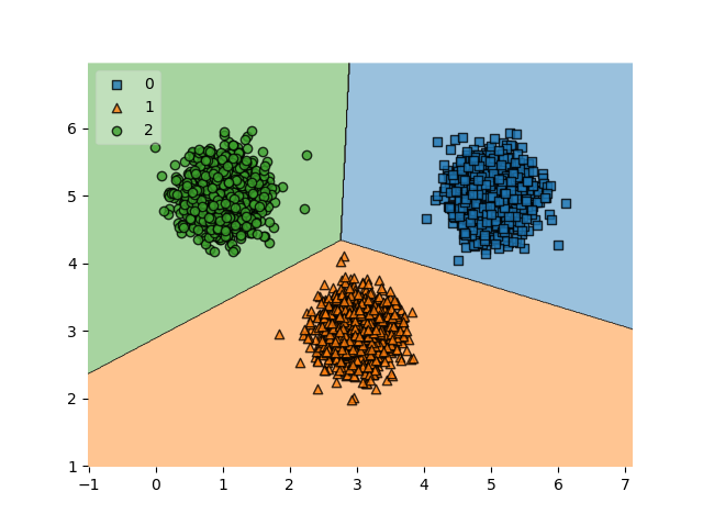
As said, some Machine Learning algorithms - like the ones that optimize a Neural network - can automatically generate a decision boundary between multiple classes. For Support Vector Machines, this does not work for the simple reason that SVMs don't support this natively. But why? Let's take a look at how an SVM operates.
An SVM is known as a kernel method that maximizes the margin between two classes by means of support vectors. Kernel methods mean that a so-called kernel function is used to generate a linear separation boundary between two classes by mapping the samples from the original feature space (i.e. axes) onto another one, where linear separation can be achieved. If the data is already linearly separable, like the black and white classes in the image below, separation is simple. In other cases, we must use more advanced kernel functions for this purpose.
In the figure below, we can observe three decision boundaries, namely \(H_1\), \(H_2\) and \(H_3\). But which one is best?
- Is \(H_1\) best? No, definitely not. It is not even capable of separating black and white, and is therefore not usable. We see such decision boundaries often by models that have just been initialized, which happens relatively randomly. Soon after, the decision boundary starts to shift.
- Is \(H_2\) best? Neither! Although it is capable of separating between black and white, it is only marginally so. Especially if an outlier from the black class is present, the odds are that it is not able to assign it the correct class, because it "crosses the line". While \(H_2\) is a decision boundary that works, we often see those boundaries in stages of the training process where separation has just been achieved, but where more optimal solutions are available.
- Is \(H_3\) best? Finally, yes. It is both capable of separating between the two classes and does so with an equal distance between \(H_3\) and the earliest black vectors and \(H_3\) and the earliest white vectors, which both are called support vectors. This is called a maximum margin and means that the boundary is equidistant to the two classes (Wikipedia, 2005).
Now this is why Support Vector Machines are called Support Vector Machines. We now also know how they work, i.e. by generating a maximum-margin linear decision boundary, by means of a kernel function.
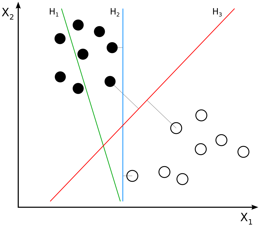
Hyperplanes and data points. The imageis not edited. Author: Zack Weinberg, derived from Cyc’s work. License: CC BY-SA 3.0
What remains unanswered is why SVMs cannot be used for multiclass classification. The answer is in fact really simple. Recall that the decision boundary must be equidistant for an SVM to converge, meaning that it must be as far as possible from both classes - and hence perfectly in the middle.
Now suppose that we add a third class and hence our decision boundary splits into three line segments, like in the green/blue/orange figure above. In this case, the line segment between blue and orange is equidistant for those two classes, but not for the green class. The same is true for the other two line segments. Since SVMs always try to find a maximum margin decision boundary, finding one for > 2 classes is impossible. This is why SVMs cannot be used for multiclass classification natively.
Fortunately, there is a solution: training multiple binary classifiers at once and using them jointly for generating a multiclass prediction. The One-vs-Rest and One-vs-One are two approaches that train multiple classifiers that compete against each other. In this article, we will continue with an interesting but different approach: that of Error-Correcting Output Codes.
Introducing Error-Correcting Output Codes
Let's recall that above, we were working on a three-class multiclass classification problem. Error-Correcting Output Codes (ECOC) represent a method for doing so by generating a variety of binary classifiers that predict output codes. In the table below, we see what is called a three-bit output code for each class. With an output code, a class can be described in some multidimensional space (in this case, a three-dimensional space). In other words, in our case, we can draw a vector \((0, 0, 1)\) in three-dimensional space in order to represent class 0. The same can be done for classes 1 and 2, making them unique.
Output codes can be used to generate a multiclass classifier, by learning a wide range of binary classifiers that predict specific bits in the output code. For example, in our three-class classification scenario, a three-bit output code is capable of describing each class. Binary classifier 3 (B3) predicts whether the input sample looks more like class 0 or like classes 1/2. B2 predicts whether the input sample looks more like class 1 or like classes 0/2. B1 predicts whether it's class 2 or classes 0/1.
By aggregating the binary classifier predictions, we get a number of bits - the output code. When generating the multiclass prediction, after aggregating the individual predictions into an output code, the predicted output code is compared to the classes available and their corresponding output code. The closest match is picked as the predicted class. This way, ECOC can be used to generate a multiclass classifier.
| Class / Classifier | B1 | B2 | B3 |
| 0 | 0 | 0 | 1 |
| 1 | 0 | 1 | 0 |
| 2 | 1 | 0 | 0 |
We haven't yet discussed why they are called error-correcting. The reason is simple. While for an N-class multiclass problem at least N binary classifiers must be trained, it is possible to train many more. For example, if we want to represent the three classes with 15-bit output codes (and hence 15 binary classifiers), this is perfectly possible. This is also what makes the method error-correcting: with each additional classifier, the output codes become more complex and therefore much more tailored to a specific class because the closest class output code is chosen.
Now, if one binary classifier is wrong, the impact would be bigger if the number of classifiers is low (e.g., a wrong prediction in the table above would immediately switch classes). If the number is high, only one out of many bits would be wrong, and the resulting output code could still be closest to the class we actually want the input to be assigned. In other words, using more binary classifiers allows them to "correct the errors of their colleagues". Of course, the more binary classifiers are added, the more resources for training are required.
Another aspect that we must cover is the initialization of the output codes. In the table above, we initialized the output codes randomly - I did not put any thought in assigning the numbers, except that the output codes must be unique. In many cases, random initialization provides adequate results. However, and especially in the case where many binary classifiers are used, better methods could exist (Scikit-learn, n.d.). It is however beyond the scope of this article to discuss them in detail.
Implementing an ECOC based SVM with Scikit-learn
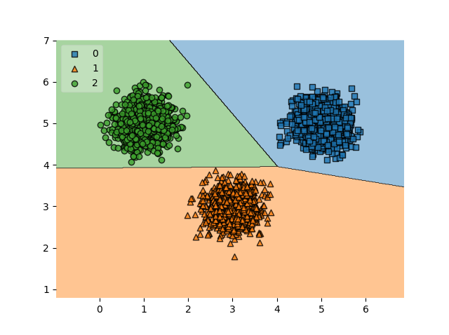
Imagine that you would need to generate a multiclass classifier for this linearly separable dataset in a two-dimensional feature space:
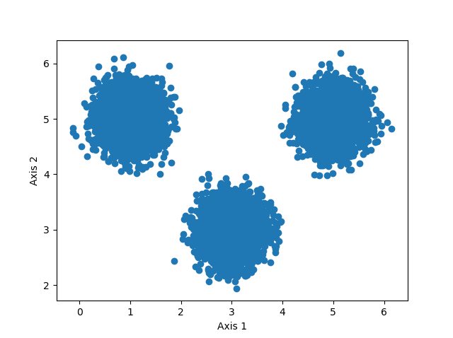
Constructing the dataset can be done in the following way:
from sklearn.datasets import make_blobs

# Configuration options
num_samples_total = 10000
cluster_centers = [(5,5), (3,3), (1,5)]
num_classes = len(cluster_centers)

# Generate data
X, y = make_blobs(n_samples = num_samples_total, centers = cluster_centers, n_features = num_classes, center_box=(0, 1), cluster_std = 0.30)
Note that for both the code above and the code below, we assume that you have installed the common data science dependencies. For today's code, they include sklearn, matplotlib, numpy and (if desired, otherwise code can be scrapped) mlxtend.
Now that we have a dataset that we can use for generating an ECOC based multiclass SVM, we can actually create our model. For creating it, we will use Scikit-learn, a widely used library for Machine Learning in Python. Let's now take a look at the code for our model and walk through it step-by-step.
- First of all, we must import all the dependencies that we need. We import
pyplotfrommatplotlibaspltfor visualizing the data, like we did above. Numpy will be used for saving the clusters if necessary; this could be useful if you want to perform model changes and run them with exactly the same generated data. We then use many functions fromsklearn. Themake_blobsfunction will be used for data generation.OutputCodeClassifieris a wrapper that makes a Scikit-learn model multiclass by adding ECOC classification.LinearSVCis a linear SVM, which is adequate for today's article since our data can be separated linearly.Train_test_splitcan be used by generating a split between training data and testing data. Withplot_confusion_matrix, we can generate a confusion matrix for our classifier. Finally, importing frommlxtend, we addplot_decision_regions, for visualizing the decision boundaries for our model. - We then specify configuration options for data generation. We create 10.000 samples around three centers, and hence have 3 classes.
- Subsequently, we generate data by calling
make_blobsfor the number of samples, centers and number of classes specified above. We set a standard deviation of 0.30 in order to make the plots only a little bit scattered, but not too much. - We then save and load the data into a
.npyfile. If you want to tune the model and train it with exactly the same data, this is useful - by simply commentingsave, you'll always use the same data. If you don't want this, you can also delete the code. - We then make the train/test split with
train_test_splitand store the split data inX_train,X_test,y_trainandy_test(i.e. the split feature vectors and corresponding labels). - We then create the
LinearSVCSVM and initialize it with some random state. - We then wrap the
svminto theOutputCodeClassifier, making it an ECOC classifier. Thecode_sizeattribute represents the "percentage of the number of classes to be used to create the code book." (Scikit-learn, n.d.) - We then fit the training data to the
ecoc_classifier, starting the training process. After fitting has completed, our trained ECOC classifier is also available inecoc_classifier, because we assign it there. - The trained classifier can then be evaluated. Performing classification analysis using a confusion matrix is a useful tool for quick-and-dirty analysis of model performance. We use
plot_confusion_matrixwith the testing data and some Matplotlib colormap to generate the confusion matrix. Withnormalize='true', we instruct Scikit to display the normalized predictions: in other words, we don't see the absolute amount of predictions on screen, but rather the proportions between predictions. - We finally plot the confusion matrix with Matplotlib.
import matplotlib.pyplot as plt
import numpy as np
from sklearn.datasets import make_blobs
from sklearn.multiclass import OutputCodeClassifier
from sklearn.svm import LinearSVC
from sklearn.model_selection import train_test_split
from sklearn.metrics import plot_confusion_matrix
from mlxtend.plotting import plot_decision_regions

# Configuration options
num_samples_total = 10000
cluster_centers = [(5,5), (3,3), (1,5)]
num_classes = len(cluster_centers)

# Generate data
X, y = make_blobs(n_samples = num_samples_total, centers = cluster_centers, n_features = num_classes, center_box=(0, 1), cluster_std = 0.30)

# Save/load data
np.save('./clusters.npy', X)
X = np.load('./clusters.npy')

# Split into training and testing data
X_train, X_test, y_train, y_test = train_test_split(X, y, test_size=0.33, random_state=42)

# Create the SVM
svm = LinearSVC(random_state=42)

# Make it an ECOC classifier
ecoc_classifier = OutputCodeClassifier(svm, code_size=6)

# Fit the data to the ECOC classifier
ecoc_classifier = ecoc_classifier.fit(X_train, y_train)

# Evaluate by means of a confusion matrix
matrix = plot_confusion_matrix(ecoc_classifier, X_test, y_test,
                                 cmap=plt.cm.Blues,
                                 normalize='true')
plt.title('Confusion matrix for ECOC classifier')
plt.show(matrix)
plt.show()

# Plot decision boundary
plot_decision_regions(X_test, y_test, clf=ecoc_classifier, legend=2)
plt.show()
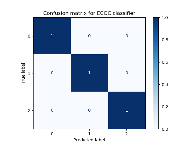
Running our code, our end result is a SVM-based linear classifier that is capable of learning a correct decision boundary. As with any perfect setting (i.e. our data is linearly separable), our confusion matrix shows great performance. Of course, in the real world, your data is likely not linearly separable and the confusion matrix will be more diffuse.
Summary
Support Vector Machines do not support multiclass classification natively. Fortunately, by using some techniques, such classifiers can be achieved - even with SVMs. In this article, we covered Error-Correcting Output Codes. These codes, which effectively map input samples to some region of a multidimensional space (and hence a class), can uniquely describe classes through multiple binary classifiers. More than the strictly required number of binary classifiers can be added, reducing the system's sensitivity to errors, making the output codes error-correcting.
We also provided an example of ECOC based multiclass classification with SVMs through the OutputCodeClassifier in Scikit-learn. In the example above, we walked through creating it step-by-step, so that you can understand in detail how such classifiers can be constructed.
I hope that you have learned something from today's article! If you did, please feel free to drop a message in the comments section below 💬 Please do the same if you have any questions or other remarks. I'd love to hear from you and will respond whenever possible. Thank you for reading MachineCurve today and happy engineering! 😎
References
Wikipedia. (2005, February 21). Equidistant. Wikipedia, the free encyclopedia. Retrieved November 11, 2020, from https://en.wikipedia.org/wiki/Equidistant
Error-Correcting Output Codes. (n.d.). https://www.ccs.neu.edu/home/vip/teach/MLcourse/4_boosting/lecture_notes/ecoc/ecoc.pdf
Scikit-learn. (n.d.). 1.12. Multiclass and multilabel algorithms — scikit-learn 0.23.2 documentation. scikit-learn: machine learning in Python — scikit-learn 0.16.1 documentation. Retrieved November 12, 2020, from https://scikit-learn.org/stable/modules/multiclass.html#error-correcting-output-codes
Scikit-learn. (n.d.). Sklearn.multiclass.OutputCodeClassifier — scikit-learn 0.23.2 documentation. scikit-learn: machine learning in Python — scikit-learn 0.16.1 documentation. Retrieved November 12, 2020, from https://scikit-learn.org/stable/modules/generated/sklearn.multiclass.OutputCodeClassifier.html#sklearn.multiclass.OutputCodeClassifier

Hi, I'm Chris!
I know a thing or two about AI and machine learning. Welcome to MachineCurve.com, where machine learning is explained in gentle terms.
Getting started
Foundation models
Learn how large language models and other foundation models are working and how you can train open source ones yourself.
Keras
Keras is a high-level API for TensorFlow. It is one of the most popular deep learning frameworks.
Machine learning theory
Read about the fundamentals of machine learning, deep learning and artificial intelligence.
Most recent articles
January 2, 2024
What is Retrieval-Augmented Generation?
December 27, 2023
In-Context Learning: what it is and how it works
December 22, 2023
CLIP: how it works, how it's trained and how to use it
Article tags
Most popular articles
February 18, 2020
How to use K-fold Cross Validation with TensorFlow 2 and Keras?
December 28, 2020
Introduction to Transformers in Machine Learning
December 27, 2021
StyleGAN, a step-by-step introduction
July 17, 2019
This Person Does Not Exist - how does it work?
October 26, 2020
Your First Machine Learning Project with TensorFlow 2.0 and Keras
Connect on social media
Connect with me on LinkedIn
To get in touch with me, please connect with me on LinkedIn. Make sure to write me a message saying hi!
Side info
The content on this website is written for educational purposes. In writing the articles, I have attempted to be as correct and precise as possible. Should you find any errors, please let me know by creating an issue or pull request in this GitHub repository.
All text on this website written by me is copyrighted and may not be used without prior permission. Creating citations using content from this website is allowed if a reference is added, including an URL reference to the referenced article.
If you have any questions or remarks, feel free to get in touch.
TensorFlow, the TensorFlow logo and any related marks are trademarks of Google Inc.
PyTorch, the PyTorch logo and any related marks are trademarks of The Linux Foundation.
Montserrat and Source Sans are fonts licensed under the SIL Open Font License version 1.1.
Mathjax is licensed under the Apache License, Version 2.0.
