How to predict new samples with your TensorFlow / Keras model?
February 21, 2020 by Chris
Training machine learning models can be awesome if they are accurate. However, you then also want to use them in production.
But how to do so?
The first step is often to allow the models to generate new predictions, for data that you - instead of Keras - feeds it.
This blog zooms in on that particular topic. By providing a Keras based example using TensorFlow 2.0+, it will show you how to create a Keras model, train it, save it, load it and subsequently use it to generate new predictions. It's the first step of deploying your model into a production setting :)
Are you ready? Let's go! 😎
Update 11/Jan/2021: added quick example to the article.
Update 03/Nov/2020: fixed textual error.
Example code: using model.predict() for predicting new samples
With this example code, you can start using model.predict() straight away.
# File path
filepath = './path_to_model'

# Load the model
model = load_model(filepath, compile = True)

# A few random samples
use_samples = [5, 38, 3939, 27389]
samples_to_predict = []

# Convert into Numpy array
samples_to_predict = np.array(samples_to_predict)

# Generate predictions for samples
predictions = model.predict(samples_to_predict)
print(predictions)
Today's Keras model
Let's first take a look at the Keras model that we will be using today for showing you how to generate predictions for new data.
It's an adaptation of the Convolutional Neural Network that we trained to demonstrate how sparse categorical crossentropy loss works. Today's one works for TensorFlow 2.0 and the integrated version of Keras; hence, I'd advise to use this variant instead of the traditional keras package.
Now, I won't cover all the steps describing how this model is built - take a look at the link above if you wish to understand this in more detail. However, very briefly:
- The model loads data from the EMNIST Digits dataset, which contains many samples of digits 0 to 9. To do this, we use our Extra Keras Datasets package.
- It prepares the data by reshaping it (adding the number of channels, which Keras requires), casting the data into the
float32type, and scaling. - It creates the ConvNet architecture: three convolutional blocks with Max Pooling for spatial hierarchy and Dropout against overfitting. Using Flatten, and Dense layers that end with a Softmax activation, we get a multiclass probability distribution.
- It compiles the model and fits the data.
- Finally, it evaluates the model based on the test set.
Here's the code - add it to a file called e.g. keras-predictions.py:
from tensorflow.keras.models import Sequential
from tensorflow.keras.layers import Dense, Dropout, Flatten
from tensorflow.keras.layers import Conv2D, MaxPooling2D
from tensorflow.keras.losses import sparse_categorical_crossentropy
from tensorflow.keras.optimizers import Adam
from extra_keras_datasets import emnist

# Model configuration
img_width, img_height = 28, 28
batch_size = 250
no_epochs = 25
no_classes = 10
validation_split = 0.2
verbosity = 1

# Load EMNIST dataset
(input_train, target_train), (input_test, target_test) = emnist.load_data(type='digits')

# Reshape data
input_train = input_train.reshape(input_train.shape[0], img_width, img_height, 1)
input_test = input_test.reshape(input_test.shape[0], img_width, img_height, 1)
input_shape = (img_width, img_height, 1)

# Cast numbers to float32
input_train = input_train.astype('float32')
input_test = input_test.astype('float32')

# Scale data
input_train = input_train / 255
input_test = input_test / 255

# Create the model
model = Sequential()
model.add(Conv2D(32, kernel_size=(3, 3), activation='relu', input_shape=input_shape))
model.add(MaxPooling2D(pool_size=(2, 2)))
model.add(Dropout(0.25))
model.add(Conv2D(64, kernel_size=(3, 3), activation='relu'))
model.add(MaxPooling2D(pool_size=(2, 2)))
model.add(Dropout(0.25))
model.add(Flatten())
model.add(Dense(256, activation='relu'))
model.add(Dense(no_classes, activation='softmax'))

# Compile the model
model.compile(loss=sparse_categorical_crossentropy,
              optimizer=Adam(),
              metrics=['accuracy'])

# Fit data to model
model.fit(input_train, target_train,
          batch_size=batch_size,
          epochs=no_epochs,
          verbose=verbosity,
          validation_split=validation_split)

# Generate generalization metrics
score = model.evaluate(input_test, target_test, verbose=0)
print(f'Test loss: {score[0]} / Test accuracy: {score[1]}')
Saving and loading the model
If we want to generate new predictions for future data, it's important that we save the model. It really is: if you don't, you'd have to retrain the model every time you want to use it. This is bad for two reasons: if you have data at scale, this is a terrible process, and your models may no longer be comparable.
Let's thus find a way to save our model!
Fortunately, Keras offers a built-in facility for saving your models. Today, we do so using the new TensorFlow SavedModel approach. However, the former way of working is also still available. Check out this post if you wish to check out saving models using both approaches in more detail.
Saving
Now, let's add some extra code to your model so that we can save and load the model :)
First, add the save_model and load_model definitions to our imports - replace the line where you import Sequential with:
from tensorflow.keras.models import Sequential, save_model, load_model
Then, create a folder in the folder where your keras-predictions.py file is stored. Make sure to name this folder saved_model or, if you name it differently, change the code accordingly - because you next add this at the end of your model file:
# Save the model
filepath = './saved_model'
save_model(model, filepath)
In line with how saving Keras models works, it saves the model instance at the filepath (i.e. that folder) that you specified.
Hooray! We now saved our trained model 🎉
Loading
Loading the model for future usage is really easy - it's a two-line addition:
# Load the model
model = load_model(filepath, compile = True)
Your model is now re-loaded from filepath and compiled automatically (i.e., the model.compile step is performed; you can also do this manually if you like).
Note that saving and loading your model during run-time of one Python file makes no sense at all: why would you write a model to your file system and load it in the same run? Yeah, you're right :) The goal is however to make your model re-usable across many Python files. Hence, in any practical setting, you'd use save_model during the training run, while you'd use load_model in e.g. another script.
Generating predictions
With a loaded model, it's time to show you how to generate predictions with your Keras model! :)
Firstly, let's add Matplotlib to our imports - which allows us to generate visualizations. Then, also add Numpy, for number processing:
import matplotlib.pyplot as plt
import numpy as np
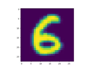
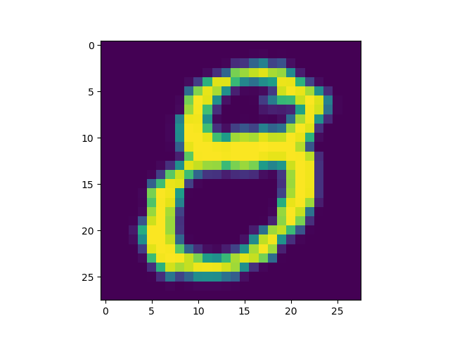
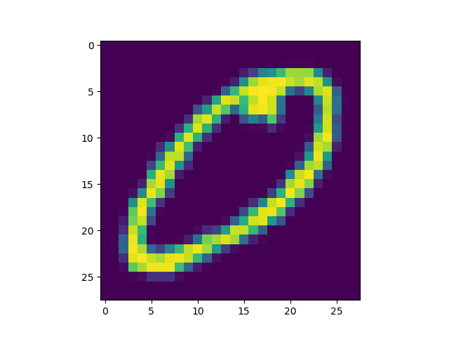
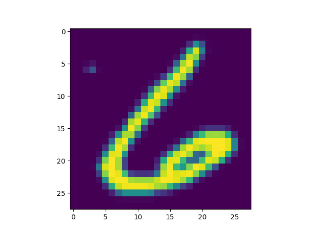
Then, we'll add some code for visualizing the samples that we'll be using in today's post:
# A few random samples
use_samples = [5, 38, 3939, 27389]

# Generate plots for samples
for sample in use_samples:
  # Generate a plot
  reshaped_image = input_train[sample].reshape((img_width, img_height))
  plt.imshow(reshaped_image)
  plt.show()
Here they are:
We then extend this code so that we can actually store the samples temporarily for prediction later:
# A few random samples
use_samples = [5, 38, 3939, 27389]
samples_to_predict = []

# Generate plots for samples
for sample in use_samples:
  # Generate a plot
  reshaped_image = input_train[sample].reshape((img_width, img_height))
  plt.imshow(reshaped_image)
  plt.show()
  # Add sample to array for prediction
  samples_to_predict.append(input_train[sample])
Then, before feeding them to the model, we convert our list into a Numpy array. This allows us to compute shape and allows Keras to handle the data more smoothly:
# Convert into Numpy array
samples_to_predict = np.array(samples_to_predict)
print(samples_to_predict.shape)
The output of the print statement: (4, 28, 28, 1).
Correct ✅ We indeed added 4 images of 28x28 pixels with one channel per image.
The next step is to generate the predictions:
# Generate predictions for samples
predictions = model.predict(samples_to_predict)
print(predictions)
The output here seems to be a bit jibberish at first:
[[8.66183618e-05 1.06925681e-05 1.40683464e-04 4.31487868e-09
  7.31811961e-05 6.07917445e-06 9.99673367e-01 7.10965661e-11
  9.43153464e-06 1.98050812e-10]
 [6.35617238e-04 9.08200348e-10 3.23482091e-05 4.98994159e-05
  7.29685112e-08 4.77315152e-05 4.25152575e-06 4.23201502e-10
  9.98981178e-01 2.48882337e-04]
 [9.99738038e-01 3.85520025e-07 1.05982785e-04 1.47284098e-07
  5.99268958e-07 2.26216093e-06 1.17733900e-04 2.74483864e-05
  3.30203284e-06 4.03360673e-06]
 [3.42538192e-06 2.30619257e-09 1.29460409e-06 7.04832928e-06
  2.71432992e-08 1.95419183e-03 9.96945918e-01 1.80040043e-12
  1.08795590e-03 1.78136176e-07]]
Confused? 😕 Don't be!
Remember that we used the Softmax activation function when creating our model. This activation function doesn't compute the prediction, but rather a discrete probability distribution over the target classes. In simple English, this means that Softmax computes the probability that the input belongs to a particular class, for each class. The values in each row summate to 1 - or 100%, which is a characteristic of a valid probability distribution.
Now, we can finalize our work by actually finding out what our predicted classes are - by taking the argmax values (or "maximum argument", index of the maximum value) for each element in the list with predictions:
# Generate arg maxes for predictions
classes = np.argmax(predictions, axis = 1)
print(classes)
This outputs [6 8 0 6]. Yeah! ✅ 🎉
Note that the code above trains with and predicts with both the training data. While this is bad practice when evaluating a model, it is acceptable when you're confident that your model generalizes to new data. I indeed am that it will generalize to new MNIST-like data, and hence I didn't make the split here.
Full code
If you're interested, you can find the code as a whole here:
from tensorflow.keras.datasets import mnist
from tensorflow.keras.models import Sequential, save_model, load_model
from tensorflow.keras.layers import Dense, Dropout, Flatten
from tensorflow.keras.layers import Conv2D, MaxPooling2D
from tensorflow.keras.losses import sparse_categorical_crossentropy
from tensorflow.keras.optimizers import Adam
from extra_keras_datasets import emnist
import matplotlib.pyplot as plt
import numpy as np

# Model configuration
img_width, img_height = 28, 28
batch_size = 250
no_epochs = 25
no_classes = 10
validation_split = 0.2
verbosity = 1

# Load EMNIST dataset
(input_train, target_train), (input_test, target_test) = emnist.load_data(type='digits')

# Reshape data
input_train = input_train.reshape(input_train.shape[0], img_width, img_height, 1)
input_test = input_test.reshape(input_test.shape[0], img_width, img_height, 1)
input_shape = (img_width, img_height, 1)

# Cast numbers to float32
input_train = input_train.astype('float32')
input_test = input_test.astype('float32')

# Scale data
input_train = input_train / 255
input_test = input_test / 255

# Create the model
model = Sequential()
model.add(Conv2D(32, kernel_size=(3, 3), activation='relu', input_shape=input_shape))
model.add(MaxPooling2D(pool_size=(2, 2)))
model.add(Dropout(0.25))
model.add(Conv2D(64, kernel_size=(3, 3), activation='relu'))
model.add(MaxPooling2D(pool_size=(2, 2)))
model.add(Dropout(0.25))
model.add(Flatten())
model.add(Dense(256, activation='relu'))
model.add(Dense(no_classes, activation='softmax'))

# Compile the model
model.compile(loss=sparse_categorical_crossentropy,
              optimizer=Adam(),
              metrics=['accuracy'])

# Fit data to model
model.fit(input_train, target_train,
          batch_size=batch_size,
          epochs=no_epochs,
          verbose=verbosity,
          validation_split=validation_split)

# Generate generalization metrics
score = model.evaluate(input_test, target_test, verbose=0)
print(f'Test loss: {score[0]} / Test accuracy: {score[1]}')

# # Save the model
filepath = './saved_model'
save_model(model, filepath)

# Load the model
model = load_model(filepath, compile = True)

# A few random samples
use_samples = [5, 38, 3939, 27389]
samples_to_predict = []

# Generate plots for samples
for sample in use_samples:
  # Generate a plot
  reshaped_image = input_train[sample].reshape((img_width, img_height))
  plt.imshow(reshaped_image)
  plt.show()
  # Add sample to array for prediction
  samples_to_predict.append(input_train[sample])

# Convert into Numpy array
samples_to_predict = np.array(samples_to_predict)
print(samples_to_predict.shape)

# Generate predictions for samples
predictions = model.predict(samples_to_predict)
print(predictions)

# Generate arg maxes for predictions
classes = np.argmax(predictions, axis = 1)
print(classes)
Summary
In today's blog post, we looked at how to generate predictions with a Keras model. We did so by coding an example, which did a few things:
- Load EMNIST digits from the Extra Keras Datasets module.
- Prepare the data.
- Define and train a Convolutional Neural Network for classification.
- Save the model.
- Load the model.
- Generate new predictions with the loaded model and validate that they are correct.
I hope you've learnt something from today's post, even though it was a bit smaller than usual :) Please let me know in the comments section what you think 💬
Thank you for reading MachineCurve today and happy engineering! 😎
References
MachineCurve. (2020, January 10). Making more datasets available for Keras. Retrieved from https://www.machinecurve.com/index.php/2020/01/10/making-more-datasets-available-for-keras/
MachineCurve. (2020, February 11). How to use sparse categorical crossentropy in Keras? Retrieved from https://www.machinecurve.com/index.php/2019/10/06/how-to-use-sparse-categorical-crossentropy-in-keras/
Cohen, G., Afshar, S., Tapson, J., & van Schaik, A. (2017). EMNIST: an extension of MNIST to handwritten letters. Retrieved from http://arxiv.org/abs/1702.05373

Hi, I'm Chris!
I know a thing or two about AI and machine learning. Welcome to MachineCurve.com, where machine learning is explained in gentle terms.
Getting started
Foundation models
Learn how large language models and other foundation models are working and how you can train open source ones yourself.
Keras
Keras is a high-level API for TensorFlow. It is one of the most popular deep learning frameworks.
Machine learning theory
Read about the fundamentals of machine learning, deep learning and artificial intelligence.
Most recent articles
January 2, 2024
What is Retrieval-Augmented Generation?
December 27, 2023
In-Context Learning: what it is and how it works
December 22, 2023
CLIP: how it works, how it's trained and how to use it
Article tags
Most popular articles
February 18, 2020
How to use K-fold Cross Validation with TensorFlow 2 and Keras?
December 28, 2020
Introduction to Transformers in Machine Learning
December 27, 2021
StyleGAN, a step-by-step introduction
July 17, 2019
This Person Does Not Exist - how does it work?
October 26, 2020
Your First Machine Learning Project with TensorFlow 2.0 and Keras
Connect on social media
Connect with me on LinkedIn
To get in touch with me, please connect with me on LinkedIn. Make sure to write me a message saying hi!
Side info
The content on this website is written for educational purposes. In writing the articles, I have attempted to be as correct and precise as possible. Should you find any errors, please let me know by creating an issue or pull request in this GitHub repository.
All text on this website written by me is copyrighted and may not be used without prior permission. Creating citations using content from this website is allowed if a reference is added, including an URL reference to the referenced article.
If you have any questions or remarks, feel free to get in touch.
TensorFlow, the TensorFlow logo and any related marks are trademarks of Google Inc.
PyTorch, the PyTorch logo and any related marks are trademarks of The Linux Foundation.
Montserrat and Source Sans are fonts licensed under the SIL Open Font License version 1.1.
Mathjax is licensed under the Apache License, Version 2.0.


