Pure signals only exist in theory. That is, when you're doing signal processing related activities, it's very likely that you'll experience noise. Whether noise is caused by the measurement (or reception) device or by the medium in which you perform measurements, you want it gone.

Various mathematical tricks exist to filter out noise from a signal. When noise is relatively constant across a range of signals, for example, you can take the mean of all the signals and deduct it from each individual signal - which likely removes the factors that contribute from noise.

However, these tricks work by knowing a few things about the noise up front. In many cases, the exact shape of your noise is unknown or cannot be estimated because it is relatively hidden. In those cases, the solution may lie in learning the noise from example data.

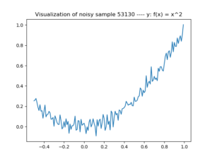
A noisy \(x^2\) sample. We'll try to remove the noise with an autoencoder.

Autoencoders can be used for this purpose. By feeding them noisy data as inputs and clean data as outputs, it's possible to make them recognize the ideosyncratic noise for the training data. This way, autoencoders can serve as denoisers.

But what are autoencoders exactly? And why does the way they work make them suitable for noise removal? And how to implement one for signal denoising / noise reduction?

We'll answer these questions in today's blog. First, we'll provide a recap on autoencoders - to (re)gain a theoretical understanding of what they are and how they work. This includes a discussion on why they can be applied to noise removal. Subsequently, we implement an autoencoder to demonstrate this, by means of a three-step process:

• We generate a large dataset of \(x^2\) samples.
• We generate a large dataset of \(x^2\) samples to which Gaussian (i.e., random) noise has been added.
• We create an autoencoder which learns to transform noisy \(x^2\) inputs into the original sine, i.e. which removes the noise - also for new data!

Ready?

Okay, let's go! 😊

Update 06/Jan/2021: updated the article to reflect TensorFlow in 2021. As 1-dimensional transposed convolutions are available in TensorFlow now, the article was updated to use Conv1D and Conv1DTranspose layers instead of their 2D variants. This fits better given the 1D aspect of our dataset. In addition, references to old Keras were replaced with newer tf.keras versions, meaning that this article is compatible with TensorFlow 2.4.0+.

Recap: what are autoencoders?

If we're going to build an autoencoder, we must know what they are.

In our blog post "Conv2DTranspose: using 2D transposed convolutions with Keras", we already covered the high-level principles behind autoencoders, but it's wise to repeat them here.

We can visualize the flow of an autoencoder as follows:

Autoencoders are composed of two parts: an encoder, which encodes some input into encoded state, and a decoder which can decode the encoded state into another format. This can be a reconstruction of the original input, as we can see in the plot below, but it can also be something different.

When autoencoders are used to reconstruct inputs from an encoded state.

For example, autoencoders are learnt for noise removal, but also for dimensionality reduction (Keras Blog , n.d.; we then use them to convert the input data into low-dimensional format, which might benefit training lower-dimensionality model types such as SVMs).

Note that the red parts in the block above - that is, the encoder and the decoder, are learnt based on data (Keras Blog, n.d.). This means that, contrary to more abstract mathematical functions (e.g. filters), they are highly specialized in one domain (e.g. signal noise removal at \(x^2\) plots as we will do next) while they perform very poorly in another (e.g. when using the same autoencoder for image noise removal).

Why autoencoders are applicable to noise removal

Autoencoders learn an encoded state with an encoder, and learn to decode this state into something else with a decoder.

Now think about this in the context of signal noise: suppose that you feed the neural network noisy data as features, while you have the pure data available as targets. Following the drawing above, the neural network will learn an encoded state based on the noisy image, and will attempt to decode it to best match the pure data. What's the thing that stands in between the pure data and the noisy data? Indeed, the noise. In effect, the autoencoder will thus learn to recognize noise and remove it from the input image.

Let's now see if we can create such an autoencoder with Keras.

Today's example: a Keras based autoencoder for noise removal

In the next part, we'll show you how to use the Keras deep learning framework for creating a denoising or signal removal autoencoder. Here, we'll first take a look at two things - the data we're using as well as a high-level description of the model.

The data

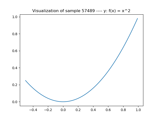
First, the data. As pure signals (and hence autoencoder targets), we're using pure \(x^2\) samples from a small domain. When plotted, a sample looks like this:

For today's model, we use 100.000 samples. To each of them, we add Gaussian noise - or random noise. While the global shape remains present, it's clear that the plots become noisy:

The model

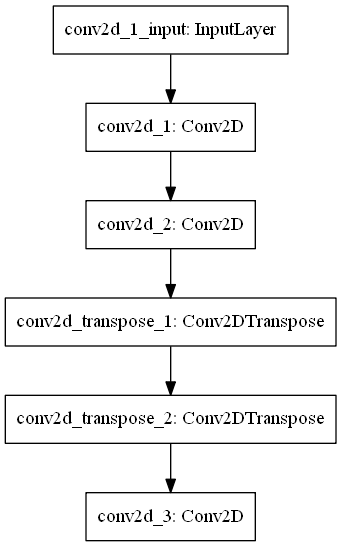
Now, the model. It looks as follows:

...and has these layers:

• The input layer, which takes the input data;
• Two Conv1D layers, which serve as encoder;
• Two Conv1D transpose layers, which serve as decoder;
• One Conv1D layer with one output, a Sigmoid activation function and padding, serving as the output layer.

To provide more details, this is the model summary:

Model: "sequential"
_________________________________________________________________
Layer (type)                 Output Shape              Param #
=================================================================
conv1d (Conv1D)              (None, 148, 128)          512
_________________________________________________________________
conv1d_1 (Conv1D)            (None, 146, 32)           12320
_________________________________________________________________
conv1d_transpose (Conv1DTran (None, 148, 32)           3104
_________________________________________________________________
conv1d_transpose_1 (Conv1DTr (None, 150, 128)          12416
_________________________________________________________________
conv1d_2 (Conv1D)            (None, 150, 1)            385
=================================================================
Total params: 28,737
Trainable params: 28,737
Non-trainable params: 0

Let's now start with the first part - generating the pure waveforms! Open up your Explorer, navigate to some folder (e.g. keras-autoencoders) and create a file called signal_generator.py. Next, open this file in your code editor - and let the coding process begin!

Generating pure waveforms

Generating pure waveforms consists of the following steps, in order to generate visualizations like the one shown on the right:

• Adding the necessary imports to the start of your Python script;
• Defining configuration settings for the signal generator;
• Generating the data, a.k.a. the pure waveforms;
• Saving the waveforms and visualizing a subset of them.

Adding imports

First, the imports - it's a simple list:

import matplotlib.pyplot as plt
import numpy as np

We use Numpy for data generation & processing and Matplotlib for visualizing some of the samples at the end.

Configuring the generator

Generator configuration consists of three steps: sample-wide configuration, intra-sample configuration and other settings. First, sample-wide configuration, which is just the number of samples to generate:

# Sample configuration
num_samples = 100000

Followed by intra-sample configuration:

# Intrasample configuration
num_elements = 1
interval_per_element = 0.01
total_num_elements = int(num_elements / interval_per_element)
starting_point = int(0 - 0.5*total_num_elements)

num_elements represents the width of your domain. interval_per_element represents the step size that the iterator will take when generating the sample. In this case, the domain \((0, 1]\) will thus contain 100 samples (as \(1/interval per element = 1/0.01 = 100\)). That's what's represented in total_num_elements.

The starting point determines where to start the generation process.

Finally, you can set the number of samples that you want visualized in the other configuration settings:

# Other configuration
num_samples_visualize = 1

Generating data

Next step, creating some data! 😁

We'll first specify the lists that contain our data and the sub-sample data (one sample in samples contains multiple xs and ys; when \(totalnumelements = 100\), that will be 100 of them each):

# Containers for samples and subsamples
samples = []
xs = []
ys = []

Next, the actual data generation part:

# Generate samples
for j in range(0, num_samples):
  # Report progress
  if j % 100 == 0:
    print(j)
  # Generate wave
  for i in range(starting_point, total_num_elements):
    x_val = i * interval_per_element
    y_val = x_val * x_val
    xs.append(x_val)
    ys.append(y_val)
  # Append wave to samples
  samples.append((xs, ys))
  # Clear subsample containers for next sample
  xs = []
  ys = []

We'll first iterate over every sample, determined by the range between 0 and the num_samples variable. This includes a progress report every 100 samples.

Next, we construct the wave step by step, adding the function outputs to the xs and ys variables.

Subsequently, we append the entire wave to the samples list, and clear the subsample containers for generating the next sample.

Saving & visualizing

The next step is to save the data. We do so by using Numpy's save call, and save samples to a file called ./signal_waves_medium.py.

```

Input shape

print(np.shape(np.array(samples[0][0])))

Save data to file for re-use

np.save('./signal_waves_medium.npy', samples)

Visualize a few random samples

for i in range(0, num_samples_visualize): random_index = np.random.randint(0, len(samples)-1) x_axis, y_axis = samples[random_index] plt.plot(x_axis, y_axis) plt.title(f'Visualization of sample {random_index}