When creating deep learning models, you often have to configure a learning rate when setting the model's hyperparameters, i.e. when you are configuring your neural network.

Every time you do that, you might actually wonder like me at first about this: what is a learning rate?

Why is it there? And how can you configure it?

We'll take a look at these questions in this blog post. This requires that we'll take a look at how models optimize first. We do so along the high-level machine learning process that we defined in another blog post.

Subsequently, we move on with learning rates - both how they work and what they do conceptually and what types of learning rates exist in today's deep learning engineers' toolboxes.

After reading this article, you will...

• Understand at a high level how models optimize.
• See how learning rates can be used to tune the amount of learning.
• Know what types of learning rates can be used in neural networks.

Let's go! 😊

Update 01/Mar/2021: ensure that article is up to date in 2021.

Update 01/Feb/2020: added link to Learning Rate Range Test.

How models optimize

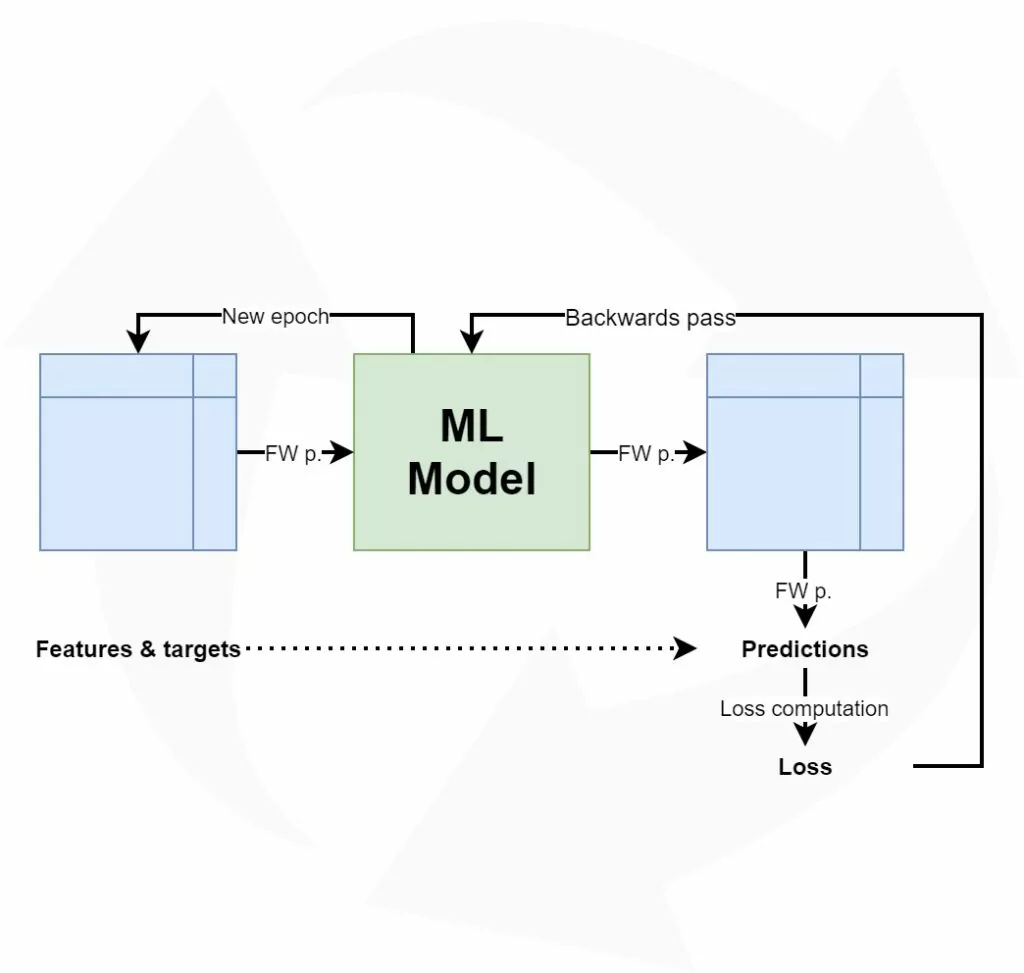
If we wish to understand what learning rates are and why they are there, we must first take a look at the high-level machine learning process for supervised learning scenarios:

Feeding data forward and computing loss

As you can see, neural networks improve iteratively. This is done by feeding the training data forward, generating a prediction for every sample fed to the model. When comparing the predictions with the actual (known) targets by means of a loss function, it's possible to determine how well (or, strictly speaking, how bad) the model performs.

Changing model weights with gradient updates

Subsequently, before starting the second iteration, the model will slightly adapt its internal structure - the weights for each neuron - by using gradients of the loss landscape. With a technique called backpropagation, the gradient of the update for a particular error is computed with respect to the original error and the neurons between the particular neuron and the error. Backprop allows you to compute the gradient efficiently by smartly using the chain rule, which you've likely encountered in calculus class.

However, this is always combined with what is known as an optimizer, which effectively performs the update. There are many optimizers: three forms of gradient descent, where you simply move in the opposite direction of the gradient, are the simplest ones. With adaptive ones, improvements to gradient descent are combined with per-neuron updates.

However - it's not a good idea that weight updates are large. This is because when weights swing back and forth, it's likely that you either have a very oscillating path towards your global minimum. Additionally, when they are large, it might be that you continously overshoot the optimum, getting worse performance than necessary!

...here's where the learning rate enters the picture 😄

Configuring how much is learnt with Learning Rates

At a highly abstract level, a weight update can be written down as follows:

new_weight = old_weight - learning rate * gradient update

You take the old weight and subtract the gradient update - but wait: you first multiply the update with the learning rate.

This learning rate, which you can configure before you start the training process, allows you to make the gradient update smaller. By default, for example in the Stochastic Gradient Descent optimizer built into the Keras deep learning framework, learning rates are relatively small - 0.01 is the default value in Keras' SGD. That essentially means that the real weights update are by default only 1% of the computed gradient update.

Yep, it'll take you longer to converge, but you likely don't overshoot and oscillate less severely across epochs!

Types of Learning Rates

The example above depicts what is known as a fixed learning rate. You set the learning rate in advance and it doesn't change over the epochs. This has both benefits and disbenefits. The primary benefit is that you have to think about your learning rate in very simple terms: you choose one number and that's it.

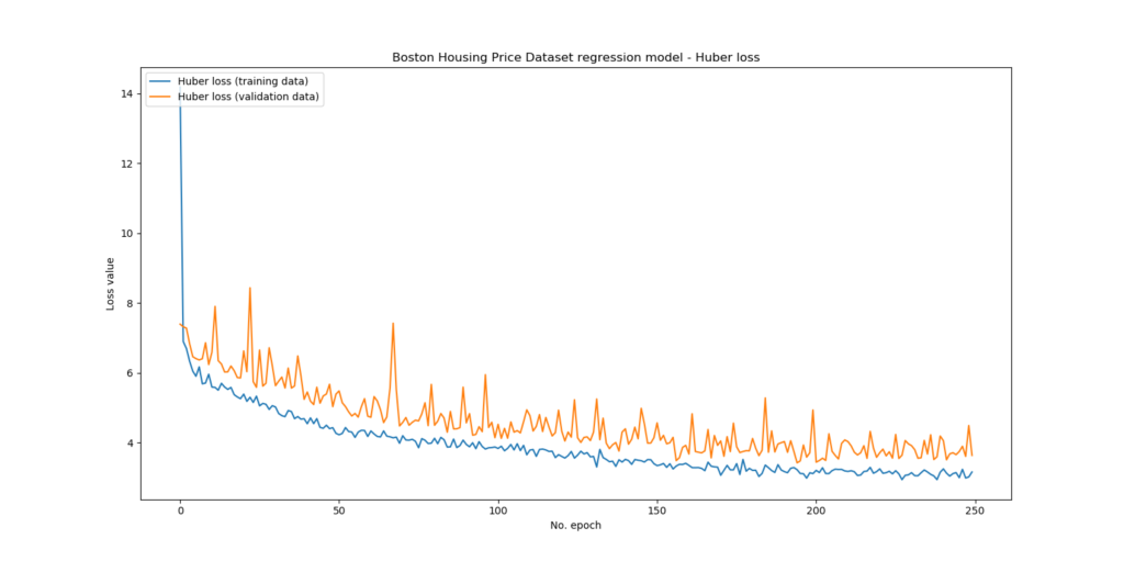
And as we shall investigate more deeply in another blog, this is also the drawback of a fixed learning rate. As you know, neural networks learn exponentially during the first few epochs - and fixed learning rates may then be too small, which means that you waste resources in terms of opportunity cost.

Loss values for some training process. As you can see, substantial learning took place initially, changing into slower learning eventually.

However, towards the more final stages of the learning process, you don't want large learning rates because the learning process slows down. Only gentle and small updates might bring you closer to the minimum, which requires small learning rates. In any other case, you may overshoot the minimum, with worse than possible performance as a result.

Enter another type of learning rate: a learning rate decay scheme. This essentially means that your learning rate gets smaller over time, allowing you to start with a relatively large one, benefiting both from the substantial improvements in the first few epochs and the more gradual ones towards the end.

There are many options here: it's possible to have your learning rate decay exponentially, linearly, or with some other function.

It's better than a fixed learning rate for obvious reasons, but learning rate decay schemes suffer from a drawback that also impacts fixed learning rates: the fact that you have to configure them in advance. This is essentially a guess, because you then don't know your exact loss landscape yet. And with any guess, the results may be good, but also disastrous.

Fortunately, there's also something as a Learning Rate Range Test, which we'll also cover in a subsequent blog. With this range test, you essentially test average model performance across a range of learning rates. This results in a plot that allows you to pick a starting learning rate based on empirical testing, which you can subsequently use in e.g. a learning rate decay scheme.

Another type of learning rate we'll cover in another blog is the concept of a Cyclical Learning Rate. In this case, the learning rate moves back and forth between a very high and a very low learning rate, in between some bounds that you can specify using the same range test as discussed previously. This is contradictory to the concept of a large learning rate at first and a small one towards the final epochs, but it actually makes a lot of sense. With larger learning rates throughout the entire training process, you can both speed up your training process in the early stages and find an escape route if you're stuck in local minima. Smaller learning rates, which will inevitably follow the larger ones, will then allow you to look around for some time, taking smaller steps towards the minimum close by. Empirical results have shown promising results.

Especially when you combine decaying learning rates and cyclical learning rates with early cutoff techniques such as EarlyStopping, it's very much possible to find a well-performing model without risking severe overfitting.

Summary

In this blog post, we've looked at the concept of a learning rate at a high level. We explained why they are there in terms of the high-level supervised machine learning process and how they are combined with feeding data forward and model optimization.

Subsequently, we looked at some types of learning rates that are available and common today: fixed learning rates, learning rate decay schemes, the Learning Rate Range Test which can be combined with either learning rate decay or Cyclical Learning Rates, which are an entirely different approach to learning.

Thanks for reading! If you have any questions or remarks, feel free to leave a comment below 👇 I'll happily answer whenever I can, and will update and/or improve my blog post if necessary.

References

Smith, L. N. (2017, March). Cyclical learning rates for training neural networks. In 2017 IEEE Winter Conference on Applications of Computer Vision (WACV) (pp. 464-472). IEEE.

Smith, L. N., & Topin, N. (2017). Exploring loss function topology with cyclical learning rates. arXiv preprint arXiv:1702.04283.

Smith, S. L., Kindermans, P. J., Ying, C., & Le, Q. V. (2017). Don't decay the learning rate, increase the batch size. arXiv preprint arXiv:1711.00489.

MachineCurve. (2019, October 22). About loss and loss functions. Retrieved from https://www.machinecurve.com/index.php/2019/10/04/about-loss-and-loss-functions/

MachineCurve. (2019, October 24). Gradient Descent and its variants. Retrieved from https://www.machinecurve.com/index.php/2019/10/24/gradient-descent-and-its-variants/

MachineCurve. (2019, November 3). Extensions to Gradient Descent: from momentum to AdaBound. Retrieved from https://www.machinecurve.com/index.php/2019/11/03/extensions-to-gradient-descent-from-momentum-to-adabound/

Jain, V. (2019, August 5). Cyclical Learning Rates ? The ultimate guide for setting learning rates for Neural Networks. Retrieved from https://medium.com/swlh/cyclical-learning-rates-the-ultimate-guide-for-setting-learning-rates-for-neural-networks-3104e906f0ae